# install.packages("motus",
#                  repos = c(birdscanada = 'https://birdscanada.r-universe.dev',
#                            CRAN = 'https://cloud.r-project.org'))
library(motus)
library(dplyr)
library(here)
library(DBI)
library(RSQLite)
library(forcats)
library(lubridate)
library(bioRad)
library(purrr)
library(ggplot2) Load & Format
Packages
You will need the motus package which you can download either online (Installing packages - Motus 2025) or from R.
Download
Note for authors:
You will have to separately run this R script that will follow the two next chunks before to continue. Indeed, `tagme( )` will prompt and require username and password that can’t be fed here.
Run this script to update database only. The procedure is heavy and takes a while to complete (up to 45 min).
# Global settings
setwd(dirname(rstudioapi::getSourceEditorContext()$path))
Sys.setenv(TZ="UTC")
proj.num <- 294
motusLogout()
First, set general settings as working directory, Time Zone and Motus project number.
Then, make sure the environment is free from any connection to any other networked project to avoid undesired mistakes.
sql.motus <- tagme(projRecv = proj.num,
                   new = FALSE, # TRUE overwrites existing file
                   update = TRUE,
                   dir = here("qmd", "chapter_1","data"))

metadata(sql.motus, proj.num)

sql.motus <- dbConnect(SQLite(), here::here("qmd", "chapter_1", "data", "project-294.motus"))

df.alltags <- tbl(sql.motus, "alltags") %>%
  dplyr::collect() %>%
  as.data.frame() %>%
    mutate(time = as_datetime(ts),
         timeAus = as_datetime(ts, tz = "Australia/Sydney"),
         dateAus = as_date(timeAus),
         year = year(time),
         doy = yday(time))
Retrieve the data from Motus server to access them in a data-frame format.
motus::tagme()gets the data from the online Motus network, the ones part of your project (ie. ID = 294) only. Make sure you set your own directory. A file of type .sql is automatically created.
If you already have a .sql file, set new = FALSE and update = TRUE so you are updating your existing file instead of re-downloading the full thing, which can take a while.
motus::metadata() downloads the metadata from the online Motus network (receiver information and more).
motus::dbConnect() links your .sql to your environment. Avoid to use high memory as .sql is a lazy table and not yet hardly written on your hardware.
motus::tbl() extracts all the tags fat into your environment. Then formatted into a classic dataframe.
tail(df.alltags %>%
       arrange(timeAus) %>%
       select(timeAus, speciesEN, motusTagID, tagModel, pulseLen, recvDeployName, recv))
timeAus speciesEN motusTagID tagModel pulseLen
3452636 2026-02-27 10:32:27 <NA> 43288 NTQB2-6-2 2.5
3452637 2026-02-27 10:32:31 <NA> 43288 NTQB2-6-2 2.5
3452638 2026-02-27 10:32:34 <NA> 43288 NTQB2-6-2 2.5
3452639 2026-02-27 10:32:37 <NA> 43288 NTQB2-6-2 2.5
3452640 2026-02-27 14:29:47 Pied Stilt 60577 NTQB2-6-2 2.5
3452641 2026-02-27 14:31:05 Pied Stilt 60577 NTQB2-6-2 2.5
recvDeployName recv
3452636 Hexham Swamp SG-010DRPI3D708
3452637 Hexham Swamp SG-010DRPI3D708
3452638 Hexham Swamp SG-010DRPI3D708
3452639 Hexham Swamp SG-010DRPI3D708
3452640 Fullerton Entrance SG-A296RPI38A7E
3452641 Fullerton Entrance SG-A296RPI38A7EAbove, a quick view about the last data uploaded to Motus server, giving you the latest detection taken into account for this workflow.
Filter
TAGS
WARNING: The values entered within the below filtering R code are depending your own context.
Here are cleaned-out the data recorded from undesired tags and/or receivers depending our local context. So the following has been processed on the raw data.
# Cleaning and correcting tags metadata
df.alltags <- df.alltags %>%
   filter(
    # test tags
     motusTagID != c("43291"),
    # pending, unconfirmed or undeployed tags
    !motusTagID %in% c("43288", "43291", "43297", "43299",
                       "43307", "43424", "43425", "60470",
                       "60579", "81123", "81136", "81137"),
    # used for test/validation before tagging bird (remove time before the tagging)
    !(motusTagID == "81134" & time < dmy("23-11-2024")),
    !(motusTagID == "60575" & time < dmy("25-10-2023")) ) %>%
    # NA species
     mutate(speciesEN = case_when(
       is.na(speciesEN) & motusTagID %in% c("60470", "81121") ~ "Red-necked Avocet",
       is.na(speciesEN) & motusTagID %in% c("81118") ~ "Red-necked Avocet",
       TRUE ~ speciesEN)) %>%

  # motusTagID as factor
  mutate(motusTagID = as.character(motusTagID))


# Cleaning and correcting receiver metadata
df.alltags <- df.alltags %>%
  filter(
    # NA
     !is.na(recvDeployLat),
    # site not any longer used
      recvDeployName != c("Throsby Creek Test Site"),
    # test sensor gnome
      recv != c("SG-C621RPI3E17F",
                "SG-62A5RPI36710") ) %>%
    # Windeyers
  mutate(recvDeployName = ifelse(is.na(recvDeployName) & recv == "SG-D5BBRPI3E2F7",
                                 "Windeyers",
                                 recvDeployName))
Have been removed:
Test tags
Tags recorded into the Motus project but undeployed;
Period of time where tags were ON but not set on any bird;
Test SensorGnome;
Sites not any longer used.
Have been modified:
Tag’s
specieENinformation have been changed from NA to different values depending case to case;Receiver station’s name
recvDeployNamehas been changed from NA to Windeyers starting from 02/15/2025.
False positive:
Let’s now visualise the quality of our data in term of False Positive and likely wrong detection because of a too low Run Length.
# Checking 'motusFiltered in' tag data
ggplot(df.alltags %>%
         filter(motusFilter == 1),
       aes(x = recvDeployName)) +
  geom_bar(fill = "steelblue") +
  theme_minimal() +
  theme(axis.text.x = element_text(angle = 45, hjust = 1)) +
labs(x = "Motus Station", y = "Nb of motusFilter = 1 (good)") 
# Checking 'motusFiltered out' tag data
ggplot(df.alltags %>%
         filter(motusFilter == 0),
       aes(x = recvDeployName)) +
  geom_bar(fill = "orange") +
  theme_minimal() +
  theme(axis.text.x = element_text(angle = 45, hjust = 1)) +
  labs(x = "Motus Station", y = "Nb of motusFilter = 0 (filtered out)")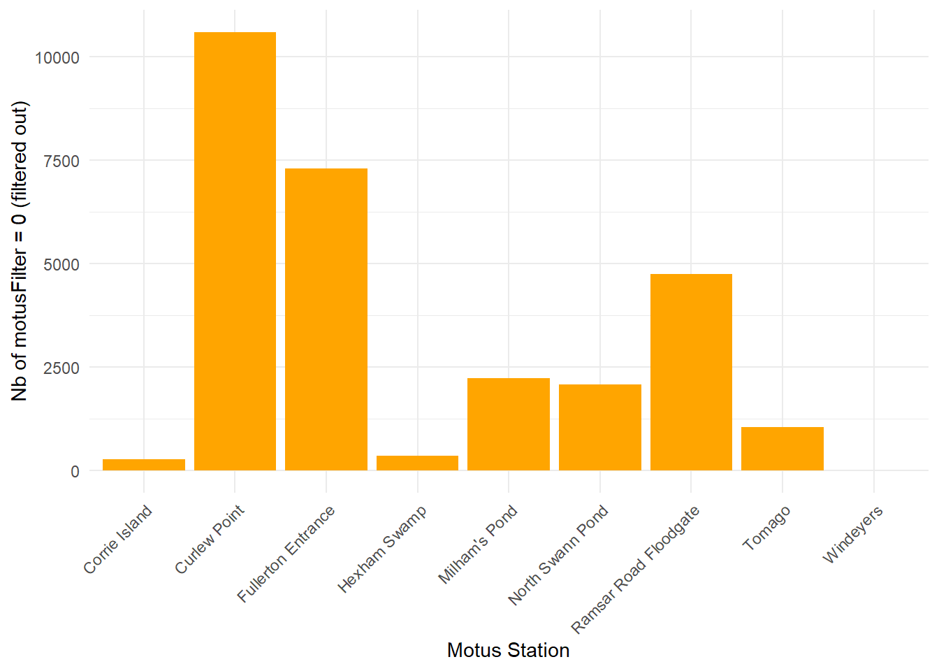
# Checking proportion of data quality for each station
perc <- ggplot(df.alltags %>%
                 filter(motusFilter %in% c(0, 1)),
       aes(x = recvDeployName, fill = factor(motusFilter))) +
  geom_bar(position = "fill") +
  scale_fill_manual(values = c("0" = "orange",
                               "1" = "steelblue"),
                    labels = c("0 (filtered out)",
                               "1 (good)"),
                    name = "motusFilter") +
  theme_minimal() +
  labs(x = "Motus Station",
       y = "Proportion") +
  scale_y_continuous(labels = scales::percent) +
  theme(axis.text.x = element_text(angle = 45, hjust = 1))

# ggpubr::ggexport(perc,
#                  filename = here("figures", "motus_filter_perc.jpg"),
#                  width = 800, height = 1000)

perc
Find in the above table the distribution of the data depending their quality and for each station.
Blue values are detections considered as True Positive from Motus and orange values as False Positive.
Indeed, a Motus station might have an interfering noisy radio environment within its vicinity (power line, flight corridor, road proximity, etc.).
Being able to flag an abnormal amount of False Positive for one station might be useful at assuming the data are True Positive but considered False Positive because of too much radio noise around.
# False positive
df.alltags <- df.alltags %>%
  filter(motusFilter == 1, # 0 is invalid data
         runLen >= 3) # value might be further thought
The False Positive signals are filtered out (i.e. noise coming from external device, or any kind of external radio activity happening within the area) thanks to the pre-made `motusFilter` and the `runLen`.
Motus Filter threshold values is set at 1, based on Motus documentationand our data (see below).
Run Length threshold value is set at 3 and defines the number of bursts recorded from one tag and received at once: too low amount of bursts are suspected to not be True Positive, therefore not reliable.
# Ambiguous
clarify(sql.motus)
[1] ambigID numHits id1 fullID1 id2 fullID2
[7] id3 fullID3 id4 fullID4 id5 fullID5
[13] id6 fullID6 motusTagID tsStart tsEnd
<0 rows> (or 0-length row.names)motus::clarify() checks whether the combination of two tag signals emitting at the mean time could generate the single detection of a third not-existing tag signal, which would also be a False Positive, but also hiding two True Positives. If the table generated by this code has rows resulting, please go to Motus documentation. A table is generated as an output and each rows correspond a case. A table with zero row means none of such a case occurred, so your data are clean.
SENSORGNOME
Receivers data and their meta-information must be filtered and formatted as well.
# Get summary
df.recvDeps <- tbl(sql.motus, "recvDeps") %>%
  collect() %>%
  as.data.frame() %>%
  mutate(timeStart = as_datetime(tsStart),
         timeStartAus = as_datetime(tsStart, tz = "Australia/Sydney"),
         timeEnd = as_datetime(tsEnd),
         timeEndAus = as_datetime(tsEnd, tz = "Australia/Sydney"))
Indeed, some receivers might have been swap within the Motus array and along time, therefore the same SensorGnome ID might be used by multiple stations along time, leading to wrong results.
IMPORTANT: Make sure you tracked the history of your receivers to avoid misled results.
Here, we only need to rename the stations accurately and to remove those that are not used any longer.
# Correct the recv names (example)
station_rename <- list("Barry_Fullerton_cove"  = "Fullerton Entrance",
                       "North Swann Pond" = "Swan Pond" ,
                       "Example_three" = "Example 3")
# Apply corrections
df.recvDeps <- df.recvDeps %>%
mutate(name = recode(name, !!!station_rename)) %>%
rename(recvDeployName = "name")
# Filter not used stations as out of the local array
df.recvDeps <- df.recvDeps %>%
filter(!is.na(latitude),
recvDeployName != c("Throsby Creek Test Site"),
serno != c("SG-C621RPI3E17F", # test station
"SG-62A5RPI36710") ) # test station# Apply corrections
df.alltags <- df.alltags %>%
mutate(recvDeployName = recode(recvDeployName, !!!station_rename))Survey time frame
df.recvDeps <- df.recvDeps %>% filter(timeStartAus > "2023-01-31 00:00:00 AEDT")Finally, we need to set temporal aspect of the survey effort.
Day one for our local Motus array to start listening any tag signals is set on the 31st January 2023 - one month before the first day a bird has been caught and tagged (information found into the SharePoint to access the file.).
Import band ID
As we might re-trap individuals and re-tag them with a new MOTUS tag, we can’t use the Motus tag ID as unique ID anymore and have to use Band ID which supposes to last on the same bird from banding date to individual’s death. Unfortunately, the Band ID is not imported by MOTUS network at the moment. So, we need to import it from our own record accessible on SharePoint here, download the .csv.
# Load df with date at the beginning
spreadsheet <- read.csv(here::here( "qmd", "chapter_1", "data", "spreadsheet", paste0(Sys.Date(), "-teams.sheet.csv"))) %>%

  # Keep only the tagged ones
  filter(Radio.tag. == "Y") %>%

  # Variable names
  rename(DateAUS.Trap = "Date",
         motusTagID = "Motus.tag.ID",
         speciesEN = "Species") %>%

  # Value names
  mutate(speciesEN = case_when(
    speciesEN == "Eastern Curlew" ~ "Far Eastern Curlew",
    speciesEN == "Black-winged Stilt" ~ "Pied Stilt",
    speciesEN == "Pacific Golden Plover" ~ "Pacific Golden-Plover",
    speciesEN == "Whimbrel" ~ "Eurasian Whimbrel",
    TRUE ~ speciesEN )) %>%

  # Format
  mutate(motusTagID = as.factor(motusTagID),
         DateAUS.Trap = as.Date(DateAUS.Trap),
         Band.ID = as.factor(Band.ID)) %>%
  select(Band.ID, motusTagID, speciesEN, DateAUS.Trap, everything())

# Format motusTagID for further merging
df.alltags <- df.alltags %>%
  mutate(motusTagID = as.factor(motusTagID))

# Join unique Band IDs for inconsistent motusTag (same bird re-tagged, etc)
df.alltags <- left_join(df.alltags,
                         spreadsheet %>%
                           filter(is.na(Euthanised.)) %>%
                           select(motusTagID, DateAUS.Trap, Band.ID, Bander),
                      by = "motusTagID")
So we merged our records with Band ID for each bird to the Motus data, linked with the Motus tag ID. Allowing unique individual IDs.
Add key variables
It is crucial for our further analysis to add the Tidal and Circadian cycles as variables so we can match each bird detection with a categorical value for a date, a tide (high/low) and a period of the day (night/day).
To do so, we must first fetch the tide data.
# Read tide.csv
tideData <- read.csv(here("qmd", "chapter_1", "data", "tides", "TideDataNewcastle.csv"))

# Format date and datetime columns
tideData <- tideData %>% mutate(
  date = dmy(date, tz = "Australia/Sydney"),
  tideDateTimeAus = dmy_hm(tideDateTimeAus, tz = "Australia/Sydney")
)

# Classify tides as diurnal or nocturnal
tideData <- tideData %>% mutate(
  sunriseNewc = sunrise(date, 151.7833, -32.9167, elev = -0.268, tz = "Australia/Sydney", force_tz = TRUE),
  sunsetNewc = sunset(date, 151.7833, -32.9167, elev = -0.268, tz = "Australia/Sydney", force_tz = TRUE),
  sunriseNewcTime = strftime(sunriseNewc, format = "%H:%M:%S", tz = "Australia/Sydney"),
  sunsetNewcTime = strftime(sunsetNewc, format = "%H:%M:%S", tz = "Australia/Sydney")
)

# Define either diurnal or nocturnal
tideData <- tideData %>% mutate(
  day_night = case_when(
    tideDateTimeAus >= sunriseNewc & tideDateTimeAus <= sunsetNewc ~ "Diurnal",
    TRUE ~ "Nocturnal"
  )
)

# Categorise each tide by tidal/diel period
tideData <- tideData %>% mutate(
    tideCategory = case_when(
      high_low == "Low" & day_night == "Diurnal" ~ "Diurnal_Low",
      high_low == "Low" & day_night == "Nocturnal" ~ "Nocturnal_Low",
      high_low == "High" & day_night == "Diurnal" ~ "Diurnal_High",
      high_low == "High" & day_night == "Nocturnal" ~ "Nocturnal_High") %>%
      as_factor())

# Add numeric ID to each category, allowing for unique tide bins
tideData <- tideData %>%
  group_by(tideCategory) %>%
  mutate(tideID = paste0(tideCategory, "_", row_number())) %>%
  ungroup()
Note that tide data-set must be extracted from New South Wales government resources and formatted into a .csv file - made for you and directly accessible here.
All the Tide categories are set for a unique point in Newcastle, easing the complexity of small scale differences for the tide within the estuary.
Let’s now add our key variables for each bird detection:
Signal strength
Circadian period
Tidal period
# Load useful functions from Callum Gapes work
tidalCurve <- readRDS(here::here("qmd", "chapter_1", "data", "tides", "tidalCurve.rds"))
tidalCurveFunc <- splinefun(tideData$tideDateTimeAus, tideData$tideHeight, method = "natural")
get.tideIndex <- function(time){ return(which.min(abs(tideData$tideDateTimeAus-time)))}

# Add key variables
df.alltags <- df.alltags  %>%

  # Positive signal strength (min. = 0) for plotting
  mutate(sigPositive = sig + abs(min(sig))) %>%

  # Sunrise/set
  sunRiseSet(lat = "recvDeployLat",
             lon = "recvDeployLon",
             ts = "ts") %>%
  mutate(sunriseNewc = sunrise(dateAus, 151.7833, -32.9167, elev = -0.268, tz = "Australia/Sydney", force_tz = TRUE),
         sunsetNewc = sunset(dateAus, 151.7833, -32.9167, elev = -0.268, tz = "Australia/Sydney", force_tz = TRUE)) %>%

  # Tide
  mutate(tideHeight = tidalCurveFunc(timeAus),
         tideIndex = map_dbl(timeAus, get.tideIndex))

  tide_values <- tideData[df.alltags$tideIndex,
                        c("tideDateTimeAus",
                          "high_low",
                          "day_night",
                          "tideCategory",
                          "tideID",
                          "tideHeight")]

# Stick and factorise the variables
df.alltags <- df.alltags %>%
  mutate(tideDateTimeAus = tide_values$tideDateTimeAus,
         tideHighLow = as_factor(tide_values$high_low),
         tideDiel = as_factor(tide_values$day_night),
         tideCategory = as_factor(tide_values$tideCategory),
         tideCategoryHeight = tide_values$tideHeight,
         tideID = as_factor(tide_values$tideID),
         tideTimeDiff = abs(difftime(timeAus, tideDateTimeAus, units = "hours")))

df.alltags <- df.alltags %>%
  mutate(Band.ID = as.factor(Band.ID))
Save
Note for authors:
Some observations (n = 11130) in the detections data retrieved from Motus server do hold NA values for speciesEN.
This can occur when tags are activated (regardless whether they are deployed on Motus server) during a catch event within the vicinity of a deployed and operational Motus station.
Catching at Curlew point on 10 March 2026 generated about 11 100 tag detections from tags we did not deployed.
These are removed from the data-set.
# Bird detection dqtq
saveRDS(df.alltags, here::here("qmd", "chapter_1", "data", "motus", paste0(Sys.Date(), "-data", ".rds" )))

# Receiver information
saveRDS(df.recvDeps, here::here("qmd", "chapter_1", "data", "motus", paste0(Sys.Date(), "-recv-info", ".rds" )))

# Spreadsheet tracking BandID
saveRDS(spreadsheet, here::here("qmd", "chapter_1", "data", "spreadsheet", paste0(Sys.Date(), "-spreadsheet", ".rds" )))

# Tide tables
saveRDS(tideData, here("qmd", "chapter_1", "data", "tides", "tideData.rds"))
Save your formatted data, now ready for analysis!
Reproducibility
Ready-to-Go!
To reproduce any of the analysis of this Research Project, simply click and download the data (a password might be required - maxime.marini@uon.edu.au).
Citation: Griffin, A. Shorebird monitoring in central NSW estuaries (Project 294). 2019. Data accessed from Motus Wildlife Tracking System, Birds Canada. Available: https://motus.org/. Accessed: YYYY-MM-DD
Once loaded in your R environment, the file will display five objects:
sql.motus: raw motus file from which you can call multiple tables (see documentation)data_all: contains all the raw detections for each Lotek nanotagsrecv: contains all the details for each receiver of the Motus arrayspreadsheet: contains all the capture events details provided for each trapped individualtideData: tidal details for Newcaslte, NSW
The data are last updated on the 21 December 2025.