library(motus)
library(dplyr)
library(here)
library(ggplot2)
library(tidyr)
library(readr)
library(dplyr)
library(ggplot2)
library(vegan)
library(philentropy)
library(gridExtra)
library(gt)
library(ggpubr)
library(car)
library(FSA)
library(patchwork)Entropy, Eveness & Composition
Load your data in your R environment - see Load & Format > Reproducibility
Shannon
Definition
Shannon entropy (H) (Shannon and Weaver -1949; MacArthur - 1965; Lou Jost - 2006)
> Is the individual site loyal?
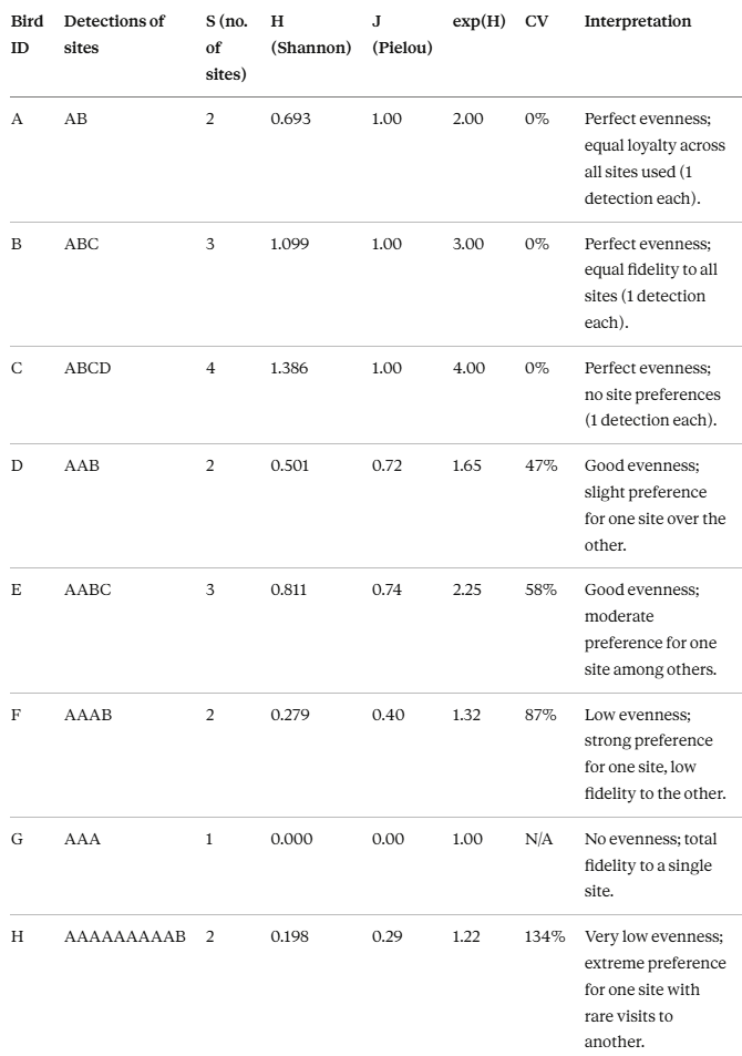
Metric employed when a large collection has a number of sites known -Type B collection (Pielou - 1966)-, to quantify the diversity of an individual’s site use. It measures the dispersion of an individual’s site use pattern.
\[ \text{H} = -Σ(p_i × ln(p_i)) \] \[ \text{where } p_i \text{ is the proportion of detections at site } i \]
- Low Entropy (e.g., H < 1.0)
Individual is highly specialized
Uses only a few sites, or uses one site predominantly
High site fidelity to specific locations
Low unpredictability: we can predict where the bird will be
- High Entropy (e.g., H > 2.0)
- Individual is generalized
- Uses many sites relatively equally
- Low site fidelity to any particular location
- High unpredictability: harder to predict where the bird will be
Coefficient of Variation (CV) (Pearson - 1984)
> Are the individuals using the same sites?
The coefficient of variation (CV) measures relative variability in site fidelity metrics, calculated as standard deviation divided by the mean (often expressed as a percentage).
- Low CV indicates uniform fidelity (e.g., most birds reuse similar site proportions)
- High CV signals heterogeneity (e.g., some wanderers vs. stayers)
Effective Number of Sites (exp(H)) (MacArthur - 1965)
> How many sites the individual is loyal to?
This transforms entropy into an interpretable number: the “effective number of equally-used sites”
\[ \text{Effective Number of Sites} = exp(H) \]
If H = 1.61, then exp(1.61) ≈ 5 effective sites. The bird uses sites as if it were splitting time equally among 5 sites (even if it actually uses 10 sites, but with uneven distribution).
Pielou’s Evenness (J) (Pielou - 1966)
> Is an individual equally loyal across the sites they are loyal to?
In practice, Shannon entropy H increases both with number of sites (Motus stations) and when site used (detections from station) become more even, so it mixes two effects. Pielou’s index rescales by dividing it by the maximum possible Shannon entropy for the same number of sites, which is ln(S) when all sites are equally represented. The resulting metric J=H/ln(S) ranges from 0 to 1 and removes the dependence on the number of sites, giving a measure of how evenly the use of sites is distributed among sites.
J close to 1: Individual uses all sites equally
J close to 0: Individual uses sites very unequally (dominates few sites)
\[ \text{J} = \frac{H}{ln(S)} \text{ where } S \text{ the total number of sites used by one individual} \]
Examples
General results
First, we define a all-in-one function to consistently computing shannon entropy.
# Function to calculate Shannon entropy
calculate_shannon <- function(proportions) {
  # Remove zero proportions (shouldn't be any, but safety check)
  p <- proportions[proportions > 0]
  # Calculate Shannon entropy: H = -sum(p * ln(p))
  H <- -sum(p * log(p))
  return(H)
}
Now we can proceed. Starting with counting the number of detection an individual has recorded in each stations, then extracting the proportions to finally calculate the entropy (H).
# Calculate entropy metrics for each Band.ID
entropy_results <- data_all %>%
  # Remove any NA values in Band.ID or recvSiteName
  filter(!is.na(Band.ID), !is.na(recvDeployName)) %>%

  # Count detections per bird per site
  group_by(speciesEN, Band.ID, recvDeployName) %>%
  summarise(detections = n(), .groups = "drop") %>%

  # Calculate proportions for each bird
  group_by(speciesEN, Band.ID) %>%
  mutate(
    total_detections = sum(detections),
    proportion = detections / total_detections) %>%

  # Calculate metrics for each bird
  summarise(
    S = n(),                                    # Number of sites used
    H = round(calculate_shannon(proportion), 2),# Shannon entropy
    J = round(H / log(S), 2),                   # Pielou's evenness
    total_detections = first(total_detections), # Total detections for reference
    .groups = "drop") %>%

  # Add effective number of equally-used sites
  mutate(
    exp_H = exp(H)) %>%

  # Arrange by Band.ID
arrange(speciesEN, Band.ID)| Table. Shannon entropy metrics for site use patterns of shorebird species in the Hunter estuary. | |||||||||||||||
|---|---|---|---|---|---|---|---|---|---|---|---|---|---|---|---|
| Species (En.) |
Sample
|
Number of Sites (S)
|
Shannon Entropy (H)
|
Pielou's Evenness (J)
|
Effective Sites [exp(H)]
|
||||||||||
| N individuals | Total detections | Median S | Mean S | SD S | Median H | Mean H | SD H | CV H (%) | Median J | Mean J | SD J | Median exp(H) | Mean exp(H) | SD exp(H) | |
| Bar-tailed Godwit | 10 | 141,008 | 2.50 | 2.20 | 0.92 | 0.42 | 0.38 | 0.34 | 87.5 | 0.60 | 0.57 | 0.28 | 1.54 | 1.54 | 0.50 |
| Curlew Sandpiper | 5 | 669,274 | 6.00 | 5.60 | 0.55 | 0.09 | 0.10 | 0.03 | 30.9 | 0.06 | 0.06 | 0.02 | 1.09 | 1.11 | 0.04 |
| Eurasian Whimbrel | 2 | 26,967 | 2.50 | 2.50 | 0.71 | 0.68 | 0.68 | 0.19 | 28.3 | 0.76 | 0.76 | 0.03 | 1.98 | 1.98 | 0.38 |
| Far Eastern Curlew | 2 | 72,927 | 2.50 | 2.50 | 0.71 | 0.36 | 0.36 | 0.45 | 125.7 | 0.34 | 0.34 | 0.40 | 1.51 | 1.51 | 0.66 |
| Masked Lapwing | 1 | 99 | 1.00 | 1.00 | NA | 0.00 | 0.00 | NA | NA | NA | NaN | NA | 1.00 | 1.00 | NA |
| Pacific Golden-Plover | 14 | 1,326,262 | 5.50 | 5.29 | 1.82 | 0.09 | 0.23 | 0.27 | 116.9 | 0.09 | 0.14 | 0.14 | 1.10 | 1.31 | 0.39 |
| Pied Stilt | 6 | 883,921 | 2.00 | 2.33 | 1.51 | 0.25 | 0.30 | 0.36 | 121.0 | 0.36 | 0.40 | 0.15 | 1.29 | 1.43 | 0.61 |
| Red-necked Avocet | 3 | 110,210 | 6.00 | 5.00 | 1.73 | 0.85 | 0.88 | 0.06 | 6.5 | 0.53 | 0.59 | 0.16 | 2.34 | 2.42 | 0.14 |
| Legend. Grouped by species, this table summarises site fidelity metrics using Shannon entropy analysis. n_individuals: number of tagged individuals; S: number of unique sites used; H: Shannon entropy (dispersion of site use, higher = more generalised); J: Pielou’s evenness (0-1, higher = more even site use); exp(H): effective number of equally-used sites; CV_H: coefficient of variation in H (% individual variation within species); total_detections: total number of detections across all individuals. Mean and standard deviation values are provided (x̄ ± SD). Median values represent the central tendency across individuals within each species. | |||||||||||||||
# Prepare data for plotting
entropy_for_plot <- entropy_results %>%
  select(speciesEN, Band.ID, S, H, J, exp_H) %>%
  pivot_longer(
    cols = c(S, H, J, exp_H),
    names_to = "metric",
    values_to = "value" ) %>%
  mutate( metric = factor(metric,
                   levels = c("S", "H", "J", "exp_H"),
                   labels = c("S (Number of Sites)",
                             "H (Shannon Entropy)",
                             "J (Pielou's Evenness)",
                             "exp(H) (Effective Sites)")))

# Create the boxplot
ggplot(entropy_for_plot, aes(x = speciesEN, y = value, fill = speciesEN)) +
  geom_boxplot(alpha = 0.7, outlier.shape = 16) +
  geom_jitter(width = 0.2, alpha = 0.3, size = 1) +
  facet_wrap(~ metric, scales = "free_y", ncol = 2) +
  scale_fill_manual(values = species_colors) +
  labs(
    title = "Shannon Entropy Metrics by Species",
    subtitle = "Distribution of site use patterns across individuals",
    x = "Species",
    y = "Value",
    fill = "Species") +
  theme_minimal() +
  theme(
    axis.text.x = element_text(angle = 45, hjust = 1, size = 9),
    strip.text = element_text(face = "bold", size = 11),
    legend.position = "none",
    panel.grid.major.x = element_blank())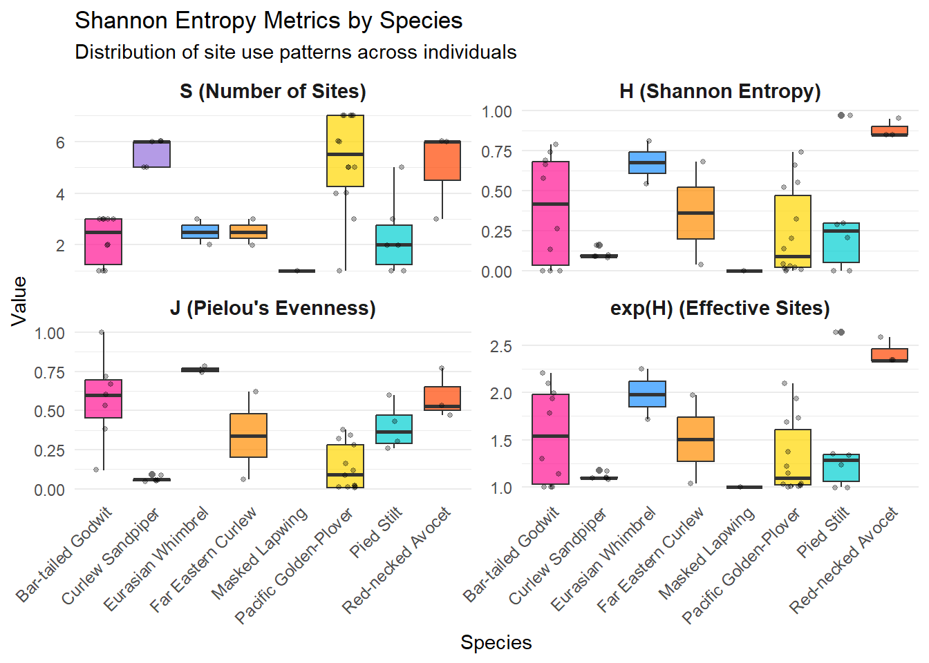
S table
| S - Number of Sites Used | ||
|---|---|---|
| Species | Band ID | S |
| Bar-tailed Godwit | 7176824 | 3 |
| Bar-tailed Godwit | 7394014 | 1 |
| Bar-tailed Godwit | 7394017 | 2 |
| Bar-tailed Godwit | 7394018 | 1 |
| Bar-tailed Godwit | 7394019 | 2 |
| Bar-tailed Godwit | 7394026 | 3 |
| Bar-tailed Godwit | 7394027 | 3 |
| Bar-tailed Godwit | 7394032 | 3 |
| Bar-tailed Godwit | 7394040 | 1 |
| Bar-tailed Godwit | 8345053 | 3 |
| Curlew Sandpiper | 4281407 | 6 |
| Curlew Sandpiper | 4281408 | 6 |
| Curlew Sandpiper | 4281409 | 5 |
| Curlew Sandpiper | 4281410 | 5 |
| Curlew Sandpiper | 4281420 | 6 |
| Eurasian Whimbrel | 8345054 | 3 |
| Eurasian Whimbrel | 8345055 | 2 |
| Far Eastern Curlew | 10118806 | 2 |
| Far Eastern Curlew | 10121744 | 3 |
| Masked Lapwing | 8295845 | 1 |
| Pacific Golden-Plover | 6318617 | 6 |
| Pacific Golden-Plover | 6318618 | 7 |
| Pacific Golden-Plover | 6318619 | 4 |
| Pacific Golden-Plover | 6318620 | 6 |
| Pacific Golden-Plover | 6318621 | 7 |
| Pacific Golden-Plover | 6318624 | 7 |
| Pacific Golden-Plover | 6318625 | 5 |
| Pacific Golden-Plover | 6318626 | 5 |
| Pacific Golden-Plover | 6318627 | 7 |
| Pacific Golden-Plover | 6318629 | 7 |
| Pacific Golden-Plover | 6318630 | 3 |
| Pacific Golden-Plover | 6318633 | 4 |
| Pacific Golden-Plover | 6318635 | 1 |
| Pacific Golden-Plover | 6318799 | 5 |
| Pied Stilt | 8295770 | 3 |
| Pied Stilt | 8295772 | 1 |
| Pied Stilt | 8295773 | 2 |
| Pied Stilt | 8295774 | 5 |
| Pied Stilt | 8295775 | 1 |
| Pied Stilt | 8295776 | 2 |
| Red-necked Avocet | 8295778 | 3 |
| Red-necked Avocet | 8295780 | 6 |
| Red-necked Avocet | 8295781 | 6 |
H table
| H - Shannon Entropy | ||
|---|---|---|
| Species | Band ID | H |
| Bar-tailed Godwit | 7176824 | 0.58 |
| Bar-tailed Godwit | 7394014 | 0.00 |
| Bar-tailed Godwit | 7394017 | 0.69 |
| Bar-tailed Godwit | 7394018 | 0.00 |
| Bar-tailed Godwit | 7394019 | 0.26 |
| Bar-tailed Godwit | 7394026 | 0.66 |
| Bar-tailed Godwit | 7394027 | 0.79 |
| Bar-tailed Godwit | 7394032 | 0.13 |
| Bar-tailed Godwit | 7394040 | 0.00 |
| Bar-tailed Godwit | 8345053 | 0.74 |
| Curlew Sandpiper | 4281407 | 0.09 |
| Curlew Sandpiper | 4281408 | 0.16 |
| Curlew Sandpiper | 4281409 | 0.08 |
| Curlew Sandpiper | 4281410 | 0.09 |
| Curlew Sandpiper | 4281420 | 0.10 |
| Eurasian Whimbrel | 8345054 | 0.81 |
| Eurasian Whimbrel | 8345055 | 0.54 |
| Far Eastern Curlew | 10118806 | 0.04 |
| Far Eastern Curlew | 10121744 | 0.68 |
| Masked Lapwing | 8295845 | 0.00 |
| Pacific Golden-Plover | 6318617 | 0.02 |
| Pacific Golden-Plover | 6318618 | 0.04 |
| Pacific Golden-Plover | 6318619 | 0.01 |
| Pacific Golden-Plover | 6318620 | 0.03 |
| Pacific Golden-Plover | 6318621 | 0.55 |
| Pacific Golden-Plover | 6318624 | 0.74 |
| Pacific Golden-Plover | 6318625 | 0.52 |
| Pacific Golden-Plover | 6318626 | 0.20 |
| Pacific Golden-Plover | 6318627 | 0.32 |
| Pacific Golden-Plover | 6318629 | 0.66 |
| Pacific Golden-Plover | 6318630 | 0.01 |
| Pacific Golden-Plover | 6318633 | 0.02 |
| Pacific Golden-Plover | 6318635 | 0.00 |
| Pacific Golden-Plover | 6318799 | 0.14 |
| Pied Stilt | 8295770 | 0.29 |
| Pied Stilt | 8295772 | 0.00 |
| Pied Stilt | 8295773 | 0.30 |
| Pied Stilt | 8295774 | 0.97 |
| Pied Stilt | 8295775 | 0.00 |
| Pied Stilt | 8295776 | 0.21 |
| Red-necked Avocet | 8295778 | 0.85 |
| Red-necked Avocet | 8295780 | 0.95 |
| Red-necked Avocet | 8295781 | 0.85 |
J table
| J - Pielou’s Evenness | ||
|---|---|---|
| Species | Band ID | J |
| Bar-tailed Godwit | 7176824 | 0.53 |
| Bar-tailed Godwit | 7394014 | NaN |
| Bar-tailed Godwit | 7394017 | 1.00 |
| Bar-tailed Godwit | 7394018 | NaN |
| Bar-tailed Godwit | 7394019 | 0.38 |
| Bar-tailed Godwit | 7394026 | 0.60 |
| Bar-tailed Godwit | 7394027 | 0.72 |
| Bar-tailed Godwit | 7394032 | 0.12 |
| Bar-tailed Godwit | 7394040 | NaN |
| Bar-tailed Godwit | 8345053 | 0.67 |
| Curlew Sandpiper | 4281407 | 0.05 |
| Curlew Sandpiper | 4281408 | 0.09 |
| Curlew Sandpiper | 4281409 | 0.05 |
| Curlew Sandpiper | 4281410 | 0.06 |
| Curlew Sandpiper | 4281420 | 0.06 |
| Eurasian Whimbrel | 8345054 | 0.74 |
| Eurasian Whimbrel | 8345055 | 0.78 |
| Far Eastern Curlew | 10118806 | 0.06 |
| Far Eastern Curlew | 10121744 | 0.62 |
| Masked Lapwing | 8295845 | NaN |
| Pacific Golden-Plover | 6318617 | 0.01 |
| Pacific Golden-Plover | 6318618 | 0.02 |
| Pacific Golden-Plover | 6318619 | 0.01 |
| Pacific Golden-Plover | 6318620 | 0.02 |
| Pacific Golden-Plover | 6318621 | 0.28 |
| Pacific Golden-Plover | 6318624 | 0.38 |
| Pacific Golden-Plover | 6318625 | 0.32 |
| Pacific Golden-Plover | 6318626 | 0.12 |
| Pacific Golden-Plover | 6318627 | 0.16 |
| Pacific Golden-Plover | 6318629 | 0.34 |
| Pacific Golden-Plover | 6318630 | 0.01 |
| Pacific Golden-Plover | 6318633 | 0.01 |
| Pacific Golden-Plover | 6318635 | NaN |
| Pacific Golden-Plover | 6318799 | 0.09 |
| Pied Stilt | 8295770 | 0.26 |
| Pied Stilt | 8295772 | NaN |
| Pied Stilt | 8295773 | 0.43 |
| Pied Stilt | 8295774 | 0.60 |
| Pied Stilt | 8295775 | NaN |
| Pied Stilt | 8295776 | 0.30 |
| Red-necked Avocet | 8295778 | 0.77 |
| Red-necked Avocet | 8295780 | 0.53 |
| Red-necked Avocet | 8295781 | 0.47 |
exp(H) table
| exp(H) - Effective Number of Sites | ||
|---|---|---|
| Species | Band ID | exp(H) |
| Bar-tailed Godwit | 7176824 | 1.79 |
| Bar-tailed Godwit | 7394014 | 1.00 |
| Bar-tailed Godwit | 7394017 | 1.99 |
| Bar-tailed Godwit | 7394018 | 1.00 |
| Bar-tailed Godwit | 7394019 | 1.30 |
| Bar-tailed Godwit | 7394026 | 1.93 |
| Bar-tailed Godwit | 7394027 | 2.20 |
| Bar-tailed Godwit | 7394032 | 1.14 |
| Bar-tailed Godwit | 7394040 | 1.00 |
| Bar-tailed Godwit | 8345053 | 2.10 |
| Curlew Sandpiper | 4281407 | 1.09 |
| Curlew Sandpiper | 4281408 | 1.17 |
| Curlew Sandpiper | 4281409 | 1.08 |
| Curlew Sandpiper | 4281410 | 1.09 |
| Curlew Sandpiper | 4281420 | 1.11 |
| Eurasian Whimbrel | 8345054 | 2.25 |
| Eurasian Whimbrel | 8345055 | 1.72 |
| Far Eastern Curlew | 10118806 | 1.04 |
| Far Eastern Curlew | 10121744 | 1.97 |
| Masked Lapwing | 8295845 | 1.00 |
| Pacific Golden-Plover | 6318617 | 1.02 |
| Pacific Golden-Plover | 6318618 | 1.04 |
| Pacific Golden-Plover | 6318619 | 1.01 |
| Pacific Golden-Plover | 6318620 | 1.03 |
| Pacific Golden-Plover | 6318621 | 1.73 |
| Pacific Golden-Plover | 6318624 | 2.10 |
| Pacific Golden-Plover | 6318625 | 1.68 |
| Pacific Golden-Plover | 6318626 | 1.22 |
| Pacific Golden-Plover | 6318627 | 1.38 |
| Pacific Golden-Plover | 6318629 | 1.93 |
| Pacific Golden-Plover | 6318630 | 1.01 |
| Pacific Golden-Plover | 6318633 | 1.02 |
| Pacific Golden-Plover | 6318635 | 1.00 |
| Pacific Golden-Plover | 6318799 | 1.15 |
| Pied Stilt | 8295770 | 1.34 |
| Pied Stilt | 8295772 | 1.00 |
| Pied Stilt | 8295773 | 1.35 |
| Pied Stilt | 8295774 | 2.64 |
| Pied Stilt | 8295775 | 1.00 |
| Pied Stilt | 8295776 | 1.23 |
| Red-necked Avocet | 8295778 | 2.34 |
| Red-necked Avocet | 8295780 | 2.59 |
| Red-necked Avocet | 8295781 | 2.34 |
Species comparison | Non-Parametric test
Important
Note: We only keep species which holds three or more individuals tagged and detected. So we can further run Kruskal-Wallis test.
Compares H and J across individuals within each species: within a species, are individuals different from each other?
# Run Kruskal-Wallis for each species separately
kruskal_within_species <- entropy_results %>%
  group_by(speciesEN) %>%
  filter(n() >= 3) %>% # minimum 3 individuals required
  summarise(
    n_individuals = n(),

    # H (Shannon Entropy)
    Chi_sq_H = kruskal.test(H ~ Band.ID)$statistic,
    df_H = kruskal.test(H ~ Band.ID)$parameter,
    p_value_H = kruskal.test(H ~ Band.ID)$p.value,

    # J (Pielou's Evenness)
    Chi_sq_J = kruskal.test(J ~ Band.ID)$statistic,
    df_J = kruskal.test(J ~ Band.ID)$parameter,
    p_value_J = kruskal.test(J ~ Band.ID)$p.value,

    # S (Number of Sites)
    Chi_sq_S = kruskal.test(S ~ Band.ID)$statistic,
    df_S = kruskal.test(S ~ Band.ID)$parameter,
    p_value_S = kruskal.test(S ~ Band.ID)$p.value,

.groups = "drop")| Within Species: Kruskal-Wallis Test Results | |||||||||||||
|---|---|---|---|---|---|---|---|---|---|---|---|---|---|
| Comparing entropy metrics across individuals within each species | |||||||||||||
| Species | N |
H (Shannon Entropy)
|
J (Pielou's Evenness)
|
S (Number of Sites)
|
|||||||||
| χ² | df | p-value | Sig. | χ² | df | p-value | Sig. | χ² | df | p-value | Sig. | ||
| Bar-tailed Godwit | 10 | 9.000 | 9 | 4.373 × 10⁻¹ | ns | 6.000 | 6 | 4.232 × 10⁻¹ | ns | 9.000 | 9 | 4.373 × 10⁻¹ | ns |
| Curlew Sandpiper | 5 | 4.000 | 4 | 4.060 × 10⁻¹ | ns | 4.000 | 4 | 4.060 × 10⁻¹ | ns | 4.000 | 4 | 4.060 × 10⁻¹ | ns |
| Pacific Golden-Plover | 14 | 13.000 | 13 | 4.478 × 10⁻¹ | ns | 12.000 | 12 | 4.457 × 10⁻¹ | ns | 13.000 | 13 | 4.478 × 10⁻¹ | ns |
| Pied Stilt | 6 | 5.000 | 5 | 4.159 × 10⁻¹ | ns | 3.000 | 3 | 3.916 × 10⁻¹ | ns | 5.000 | 5 | 4.159 × 10⁻¹ | ns |
| Red-necked Avocet | 3 | 2.000 | 2 | 3.679 × 10⁻¹ | ns | 2.000 | 2 | 3.679 × 10⁻¹ | ns | 2.000 | 2 | 3.679 × 10⁻¹ | ns |
| Significance codes: *** p < 0.001, ** p < 0.01, * p < 0.05, ns = not significant (p ≥ 0.05). N = number of individuals. Green/blue/yellow highlighting indicates significant differences among individuals within that species. Only species with ≥3 individuals are included (minimum requirement for Kruskal-Wallis test). | |||||||||||||
Tidal dependance | Parametric test
We now want to clarify whether birds associate site fidelity depending the tide, therefore likely depending their behavior (i.e., foraging vs roosting).
# Calculate entropy metrics for each Band.ID
entropy_results_tide <- data_all %>%
  # Remove any NA values in Band.ID or recvSiteName
  filter(!is.na(Band.ID), !is.na(recvDeployName)) %>%

  # Count detections per bird per site
  group_by(speciesEN, Band.ID, recvDeployName, tideHighLow) %>%
  summarise(detections = n(), .groups = "drop") %>%

  # Calculate proportions for each bird
  group_by(speciesEN, Band.ID, tideHighLow) %>%
  mutate(
    total_detections = sum(detections),
    proportion = detections / total_detections) %>%

  # Calculate metrics for each bird
  summarise(
    S = n(),                                              # Number of sites used
    H = round(calculate_shannon(proportion), 2),          # Shannon entropy
    J = round(H / log(S), 2),                             # Pielou's evenness
    total_detections = first(total_detections),           # Total detections for reference
    .groups = "drop") %>%

  # Add effective number equally-used sites
  mutate(exp_H = exp(H)) %>%

  # Arrange by Band.ID
  arrange(speciesEN, Band.ID, tideHighLow)
Let’s summarise the data accordingly to the tide. Here, we display statistical values (n, mean, sd) for each metrics related to entropy.
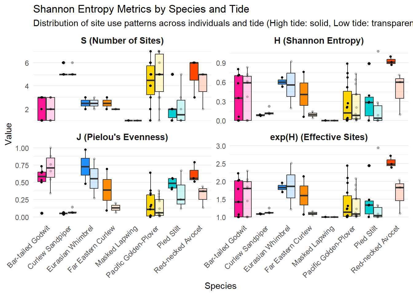
Find below for each species their associated metrics of entropy, side by side with high and low tides so it is easily comparable and reportable to the figure above.
| Table. Shannon entropy metrics for site use patterns of shorebird species by tide state in the Hunter estuary. | |||||||||||||||
|---|---|---|---|---|---|---|---|---|---|---|---|---|---|---|---|
| Tide |
Sample
|
Number of Sites (S)
|
Shannon Entropy (H)
|
Pielou's Evenness (J)
|
Effective Sites [exp(H)]
|
||||||||||
| N indiv. | Total det. | Median | Mean | SD | Median | Mean | SD | CV (%) | Median | Mean | SD | Median | Mean | SD | |
| Red-necked Avocet | |||||||||||||||
| High | 3 | 83,598 | 6.00 | 5.00 | 1.73 | 0.91 | 0.93 | 0.07 | 7.2 | 0.56 | 0.62 | 0.15 | 2.48 | 2.53 | 0.17 |
| Low | 3 | 26,612 | 5.00 | 4.00 | 1.73 | 0.60 | 0.47 | 0.33 | 70.9 | 0.37 | 0.31 | 0.16 | 1.82 | 1.65 | 0.49 |
| Pied Stilt | |||||||||||||||
| High | 6 | 492,414 | 2.00 | 2.17 | 1.47 | 0.28 | 0.31 | 0.33 | 106.2 | 0.48 | 0.48 | 0.08 | 1.33 | 1.43 | 0.53 |
| Low | 6 | 391,507 | 1.50 | 2.17 | 1.60 | 0.04 | 0.24 | 0.43 | 177.3 | 0.25 | 0.35 | 0.29 | 1.04 | 1.39 | 0.77 |
| Pacific Golden-Plover | |||||||||||||||
| High | 14 | 657,498 | 4.50 | 4.36 | 1.86 | 0.12 | 0.26 | 0.32 | 122.6 | 0.11 | 0.17 | 0.20 | 1.13 | 1.36 | 0.48 |
| Low | 14 | 668,764 | 5.00 | 4.86 | 1.96 | 0.08 | 0.23 | 0.27 | 115.6 | 0.06 | 0.14 | 0.14 | 1.08 | 1.30 | 0.38 |
| Masked Lapwing | |||||||||||||||
| High | 1 | 22 | 1.00 | 1.00 | NA | 0.00 | 0.00 | NA | NA | NA | NaN | NA | 1.00 | 1.00 | NA |
| Low | 1 | 77 | 1.00 | 1.00 | NA | 0.00 | 0.00 | NA | NA | NA | NaN | NA | 1.00 | 1.00 | NA |
| Far Eastern Curlew | |||||||||||||||
| High | 2 | 21,392 | 2.50 | 2.50 | 0.71 | 0.41 | 0.41 | 0.49 | 120.7 | 0.39 | 0.39 | 0.42 | 1.60 | 1.60 | 0.76 |
| Low | 2 | 51,535 | 2.00 | 2.00 | 0.00 | 0.09 | 0.09 | 0.07 | 78.6 | 0.13 | 0.13 | 0.10 | 1.10 | 1.10 | 0.08 |
| Eurasian Whimbrel | |||||||||||||||
| High | 2 | 15,408 | 2.50 | 2.50 | 0.71 | 0.60 | 0.60 | 0.10 | 16.5 | 0.72 | 0.72 | 0.35 | 1.83 | 1.83 | 0.18 |
| Low | 2 | 11,559 | 2.50 | 2.50 | 0.71 | 0.56 | 0.56 | 0.52 | 93.0 | 0.55 | 0.55 | 0.40 | 1.86 | 1.86 | 0.92 |
| Curlew Sandpiper | |||||||||||||||
| High | 5 | 374,495 | 5.00 | 5.20 | 0.45 | 0.08 | 0.08 | 0.01 | 10.2 | 0.05 | 0.05 | 0.01 | 1.08 | 1.09 | 0.01 |
| Low | 5 | 294,779 | 5.00 | 5.20 | 0.45 | 0.11 | 0.13 | 0.05 | 39.2 | 0.06 | 0.08 | 0.03 | 1.12 | 1.14 | 0.06 |
| Bar-tailed Godwit | |||||||||||||||
| High | 9 | 115,486 | 3.00 | 2.22 | 0.97 | 0.35 | 0.36 | 0.35 | 97.4 | 0.58 | 0.52 | 0.24 | 1.42 | 1.50 | 0.51 |
| Low | 9 | 25,522 | 2.00 | 2.11 | 0.93 | 0.59 | 0.42 | 0.34 | 80.4 | 0.71 | 0.70 | 0.24 | 1.80 | 1.60 | 0.51 |
| Legend. Grouped by species and tide state (Low/High), this table summarises site fidelity metrics using Shannon entropy analysis. tideHighLow: tide state during detections (Low or High tide); n_individuals: number of tagged individuals; S: number of unique sites used; H: Shannon entropy (dispersion of site use, higher = more generalised); J: Pielou’s evenness (0-1, higher = more even site use); exp(H): effective number of equally-used sites; CV_H: coefficient of variation in H (% individual variation within species); total_detections: total number of detections across all individuals. Mean and standard deviation values are provided (x̄ ± SD). Median values represent the central tendency across individuals within each species. | |||||||||||||||
ANOVA (Analysis of Variance) is a statistical test that compares means across groups to see if at least one group is significantly different from the others.
A two-way ANOVA examines how two categorical independent variables (tideHihghLow & Band.ID) affect a continuous dependent variable (entropy metric values).
So, we are testing three cases:
Do individual birds (Band.ID) differ in their entropy metric values? (m1, addditive model)
Do tide conditions (tideHighLow) affect entropy metric values? (m1, additive model)
Does the effect of tide vary by individual? (m2, interaction model)
Important
Note: We only keep species which holds five or more individuals tagged and detected before to run ANOVA analysis on the data.
Before to run ANOVA analysis we must check the data verify the ANOVA Assumptions.
We now set the table which will check whether the ANOVA assumptions are violated or met (ie., independence, normality and homogeneity).
By design, the data are independents: each Band.ID is a unique individual and not repeated within a tide per entropy metrics.
You will notice that we actually run the Two-Way ANOVA analysis in this same step to facilitate smoothness of the code.
results      <- data.frame()
assumptions  <- data.frame()
species_list_entropy <- unique(entropy_aov_data_tide$speciesEN)
metrics_list_entropy <- unique(entropy_aov_data_tide$metric)


for (sp in species_list_entropy) {
  for (m in metrics_list_entropy) {

    df <- subset(entropy_aov_data_tide, speciesEN == sp & metric == m)
    df <- na.omit(df)
    df$Band.ID     <- droplevels(df$Band.ID)       # drop unused factor levels
    df$tideHighLow <- droplevels(df$tideHighLow)

    model <- aov(value ~ Band.ID + tideHighLow, data = df) # ANOVA test
    s     <- summary(model)[[1]]

    # --- ANOVA results (tideHighLow row only) ---
    for (term in c("Band.ID", "tideHighLow")) {
      if (term %in% rownames(s)) {
        results <- rbind(results, data.frame(
          Species = sp,
          Metric  = as.character(m),
          Term    = ifelse(term == "tideHighLow", "Tide effect", term),
          Df      = s[term, "Df"],
          SS      = round(s[term, "Sum Sq"],  3),
          MS      = round(s[term, "Mean Sq"], 3),
          F_value = round(s[term, "F value"], 3),
          p_value = round(s[term, "Pr(>F)"],  4),
          stringsAsFactors = FALSE))
      }
    }

    # Independence
    indep_note <- "By design"

    # Normality of residuals (Shapiro-Wilk)
    res <- residuals(model)
    sw  <- shapiro.test(res)

    # Homogeneity of variance (Levene's test)
    lev <- tryCatch(
      leveneTest(value ~ tideHighLow, data = df, center = median),
      error = function(e) NULL)

    assumptions <- rbind(assumptions, data.frame(
      Species          = sp,
      Metric           = as.character(m),
      N                = nrow(df),
      Independence     = indep_note,
      SW_W             = round(sw$statistic, 4),
      SW_p             = round(sw$p.value,   4),
      Normality        = ifelse(sw$p.value > 0.049, "✓ Met", "✗ Violated"),
      Levene_F         = ifelse(!is.null(lev), round(lev$`F value`[1], 4), NA),
      Levene_p         = ifelse(!is.null(lev), round(lev$`Pr(>F)`[1],  4), NA),
      Homogeneity      = ifelse(!is.null(lev),
                           ifelse(lev$`Pr(>F)`[1] > 0.049, "✓ Met", "✗ Violated"),
                           "Insufficient levels"),
      stringsAsFactors = FALSE))
  }
}


# Prepare results sign.
results <- results %>%
  mutate(
    sig = case_when(
      p_value < 0.001 ~ "***",
      p_value < 0.01  ~ "**",
      p_value < 0.05  ~ "*",
      p_value < 0.1   ~ ".",
      TRUE            ~ ""))
Let’s plot Two-Way ANOVA assumptions outputs first.
| ANOVA Assumption Tests | ||||||||
|---|---|---|---|---|---|---|---|---|
| Normality (Shapiro-Wilk) and Homogeneity of Variance (Levene’s test) | ||||||||
| Metric | n | Independence |
Shapiro-Wilk
|
Levene's Test
|
||||
| W | p value | Normality | F | p value | Homogeneity | |||
| Bar-tailed Godwit | ||||||||
| S (Number of Sites) | 18 | By design | 0.9143 | 0.1027 | ✓ Met | 0.0000 | 1.0000 | ✓ Met |
| H (Shannon Entropy) | 18 | By design | 0.9506 | 0.4337 | ✓ Met | 0.0889 | 0.7695 | ✓ Met |
| J (Pielou's Evenness) | 12 | By design | 0.9475 | 0.6001 | ✓ Met | 0.0822 | 0.7802 | ✓ Met |
| exp(H) (Effective Sites) | 18 | By design | 0.9617 | 0.6354 | ✓ Met | 0.0492 | 0.8272 | ✓ Met |
| Curlew Sandpiper | ||||||||
| S (Number of Sites) | 10 | By design | 0.8148 | 0.0219 | ✗ Violated | 0.0000 | 1.0000 | ✓ Met |
| H (Shannon Entropy) | 10 | By design | 0.9374 | 0.5250 | ✓ Met | 1.1256 | 0.3197 | ✓ Met |
| J (Pielou's Evenness) | 10 | By design | 0.9621 | 0.8099 | ✓ Met | 0.7840 | 0.4018 | ✓ Met |
| exp(H) (Effective Sites) | 10 | By design | 0.9370 | 0.5200 | ✓ Met | 1.1354 | 0.3177 | ✓ Met |
| Pacific Golden-Plover | ||||||||
| S (Number of Sites) | 28 | By design | 0.8989 | 0.0108 | ✗ Violated | 0.0262 | 0.8726 | ✓ Met |
| H (Shannon Entropy) | 28 | By design | 0.8376 | 0.0005 | ✗ Violated | 0.1702 | 0.6833 | ✓ Met |
| J (Pielou's Evenness) | 26 | By design | 0.8201 | 0.0004 | ✗ Violated | 0.5141 | 0.4803 | ✓ Met |
| exp(H) (Effective Sites) | 28 | By design | 0.7713 | 0.0000 | ✗ Violated | 0.2207 | 0.6424 | ✓ Met |
| Pied Stilt | ||||||||
| S (Number of Sites) | 12 | By design | 0.7744 | 0.0049 | ✗ Violated | 0.2353 | 0.6381 | ✓ Met |
| H (Shannon Entropy) | 12 | By design | 0.9710 | 0.9210 | ✓ Met | 0.0177 | 0.8969 | ✓ Met |
| J (Pielou's Evenness) | 7 | By design | 0.9679 | 0.8829 | ✓ Met | 1.1353 | 0.3354 | ✓ Met |
| exp(H) (Effective Sites) | 12 | By design | 0.9430 | 0.5375 | ✓ Met | 0.0416 | 0.8425 | ✓ Met |
| Independence: verified by design — each Band.ID is a unique individual measured once per tide condition per metric. Shapiro-Wilk: H₀ = residuals are normally distributed; p > 0.05 → assumption met. Levene’s test: H₀ = variances are equal across tide groups; p > 0.05 → assumption met. |
||||||||
We can now proceed and plot the Two-Way ANOVA analysis.
# Display plot
results %>%
  gt(groupname_col = "Species", rowname_col = "Term") %>%

  tab_header(
    title    = md("**Two-Way ANOVA Results**"),
    subtitle = md("*value ~ Band.ID + tideHighLow — by Species and Metric*")) %>%

  cols_label(
    Metric  = "Metric",
    Df      = "df",
    SS      = "Sum Sq",
    MS      = "Mean Sq",
    F_value = "F value",
    p_value = "p value",
    sig     = "") %>%

  tab_style(
    style     = cell_text(weight = "bold"),
    locations = cells_body(
      columns = vars(p_value, sig),
      rows    = sig %in% c("*", "**", "***", ".") )) %>%

  opt_row_striping() %>%

  tab_source_note(
    source_note = "Significance codes: *** p<0.001  ** p<0.01  * p<0.05  . p<0.1") %>%

  tab_options(
    row_group.font.weight      = "bold",
    row_group.background.color = "#f0f4f8",
    heading.align              = "left",
table.font.size = 13 )| Two-Way ANOVA Results | |||||||
|---|---|---|---|---|---|---|---|
| value ~ Band.ID + tideHighLow — by Species and Metric | |||||||
| Metric | df | Sum Sq | Mean Sq | F value | p value | ||
| Bar-tailed Godwit | |||||||
| Tide effect | S (Number of Sites) | 1 | 0.250 | 0.250 | 2.333 | 0.1705 | |
| Tide effect | H (Shannon Entropy) | 1 | 0.000 | 0.000 | 0.008 | 0.9329 | |
| Tide effect | J (Pielou's Evenness) | 1 | 0.034 | 0.034 | 0.469 | 0.5311 | |
| Tide effect | exp(H) (Effective Sites) | 1 | 0.001 | 0.001 | 0.005 | 0.9456 | |
| Curlew Sandpiper | |||||||
| Tide effect | S (Number of Sites) | 1 | 0.000 | 0.000 | 0.000 | 1.0000 | |
| Tide effect | H (Shannon Entropy) | 1 | 0.006 | 0.006 | 5.434 | 0.0802 | . |
| Tide effect | J (Pielou's Evenness) | 1 | 0.002 | 0.002 | 4.506 | 0.1010 | |
| Tide effect | exp(H) (Effective Sites) | 1 | 0.007 | 0.007 | 4.985 | 0.0893 | . |
| Pacific Golden-Plover | |||||||
| Tide effect | S (Number of Sites) | 1 | 1.750 | 1.750 | 2.116 | 0.1695 | |
| Tide effect | H (Shannon Entropy) | 1 | 0.005 | 0.005 | 0.447 | 0.5154 | |
| Tide effect | J (Pielou's Evenness) | 1 | 0.006 | 0.006 | 0.873 | 0.3684 | |
| Tide effect | exp(H) (Effective Sites) | 1 | 0.022 | 0.022 | 0.608 | 0.4497 | |
| Pied Stilt | |||||||
| Tide effect | S (Number of Sites) | 1 | 0.000 | 0.000 | 0.000 | 1.0000 | |
| Tide effect | H (Shannon Entropy) | 1 | 0.014 | 0.014 | 0.699 | 0.4411 | |
| Tide effect | J (Pielou's Evenness) | 1 | 0.018 | 0.018 | 0.850 | 0.4539 | |
| Tide effect | exp(H) (Effective Sites) | 1 | 0.004 | 0.004 | 0.076 | 0.7944 | |
| Significance codes: *** p<0.001 ** p<0.01 * p<0.05 . p<0.1 | |||||||
Jensen-Shannon Divergence
Definition
JSD (Lin - 1991; Takahashi et al. 2012)
> Do the individuals use the same sites? Are they loyal to the same sites?
Now we know how loyal individuals are to their sites and whether there are differences across species in term of site fidelity (H), we also put against this metric the evenness which describes whether a bird use multiple site but effectively use a few (J).
We now want to clarify whether birds are using the same sites within the same species, regardless the number of sites used. We called another metric named Jensen-Shannon Divergence (JSD), which quantifies how different two probability distributions of site usage are (e.g., site proportions for two birds), answering whether two individuals are using the same composition of sites.
JSD is defined with the simplified formula here below:
\[ \text{JSD}(P∥Q) = H(M) - \frac{H(P) + H(Q)}{2} \]
\[ \text{where } Q \text{ and } P \text{ the site use distributions for two individuals; } M \text{ the mixture (average) site distribution; and } H \text{ the Shannon entropy} \]
- JSD ≈ 0 (Similarity ≈ 1.0)
- Individuals use sites in nearly identical proportions
- High overlap in site use patterns
- Suggests shared habitat preferences or social coordination
- Individuals use sites in nearly identical proportions
- JSD ≈ 1.0 (Similarity ≈ 0)
- Individuals use completely different sets of sites or proportions
- Low overlap in site use patterns
- Suggests individual specialization or territoriality
- Individuals use completely different sets of sites or proportions
General results
First, we set a function that will compute the JSD metric for later in the process.
# Function to calculate Jensen-Shannon Divergence
calculate_jsd <- function(p, q) {
  # Add small value to avoid log(0)
  epsilon <- 1e-10
  p <- p + epsilon
  q <- q + epsilon

  # Normalise
  p <- p / sum(p)
  q <- q / sum(q)

  # Calculate JSD
  m <- (p + q) / 2
  jsd <- 0.5 * sum(p * log2(p / m)) + 0.5 * sum(q * log2(q / m))

  return(jsd)
}
Second, we need to prepare the data frame which will be used for calculation. It must include for each individual its proportion of site used and its total.
Then, we can proceed and extract JSD for each pair of individuals. Indeed, JSD test the similarity between two individual, so it conducts a pairwise test.
# Create site use matrix (rows = individuals, columns = sites)
site_use_matrix <- data_all %>%
  filter(!is.na(Band.ID), !is.na(recvDeployName)) %>%
  group_by(Band.ID, recvDeployName) %>%
  summarise(detections = n(), .groups = "drop") %>%
  group_by(Band.ID) %>%
  mutate(proportion = round(detections / sum(detections), 2)) %>%
  select(Band.ID, recvDeployName, proportion) %>%
  pivot_wider(
    names_from = recvDeployName,
    values_from = proportion,
    values_fill = 0)

# Calculate pairwise JSD
individual_ids <- site_use_matrix$Band.ID
n_individuals <- length(individual_ids)

jsd_results <- data.frame()

for (i in 1:(n_individuals - 1)) {
  for (j in (i + 1):n_individuals) {

    p <- as.numeric(site_use_matrix[i, -1])
    q <- as.numeric(site_use_matrix[j, -1])

    jsd_results <- rbind(jsd_results, data.frame(
      Band.ID_1 = individual_ids[i],
      Band.ID_2 = individual_ids[j],
      JSD = round(calculate_jsd(p, q), 3), # using formula built beforehands
      Similarity = round(1 - calculate_jsd(p, q), 3)))
  }
}

# Add species information
jsd_results <- jsd_results %>%
  left_join(data_all %>% select(Band.ID, speciesEN) %>% distinct(),
            by = c("Band.ID_1" = "Band.ID")) %>%
  rename(species_1 = speciesEN) %>%
  left_join(data_all %>% select(Band.ID, speciesEN) %>% distinct(),
            by = c("Band.ID_2" = "Band.ID")) %>%
  rename(species_2 = speciesEN) %>%
  mutate(same_species = species_1 == species_2)
We can summarise the results to better handle visualisations in the below figure, and report to data in the following table.
# Filter to same_species comparisons and prepare for boxplot (matching entropy_for_plot structure)
jsd_for_plot <- jsd_results %>%

  filter(same_species == TRUE) %>%

  mutate(
    metric = "JSD",
    speciesEN = species_1) %>%

  select(speciesEN, JSD, metric) %>%
  rename(value = JSD)

# Boxplot exactly matching your entropy format
ggplot(jsd_for_plot, aes(x = speciesEN, y = value, fill = speciesEN)) +

  geom_boxplot(alpha = 0.7, outlier.shape = 16) +
  geom_jitter(width = 0.2, alpha = 0.3, size = 1) +

  scale_fill_manual(values = species_colors) +

  labs(
    title = "Jensen-Shannon Divergence by Species",
    subtitle = "Individual pairwise similarity within species",
    x = "Species",
    y = "JSD Value",
    fill = "Species") +

  theme_minimal() +
  theme(
    axis.text.x = element_text(angle = 45, hjust = 1, size = 9),
    strip.text = element_text(face = "bold", size = 11),
    legend.position = "none",
    panel.grid.major.x = element_blank())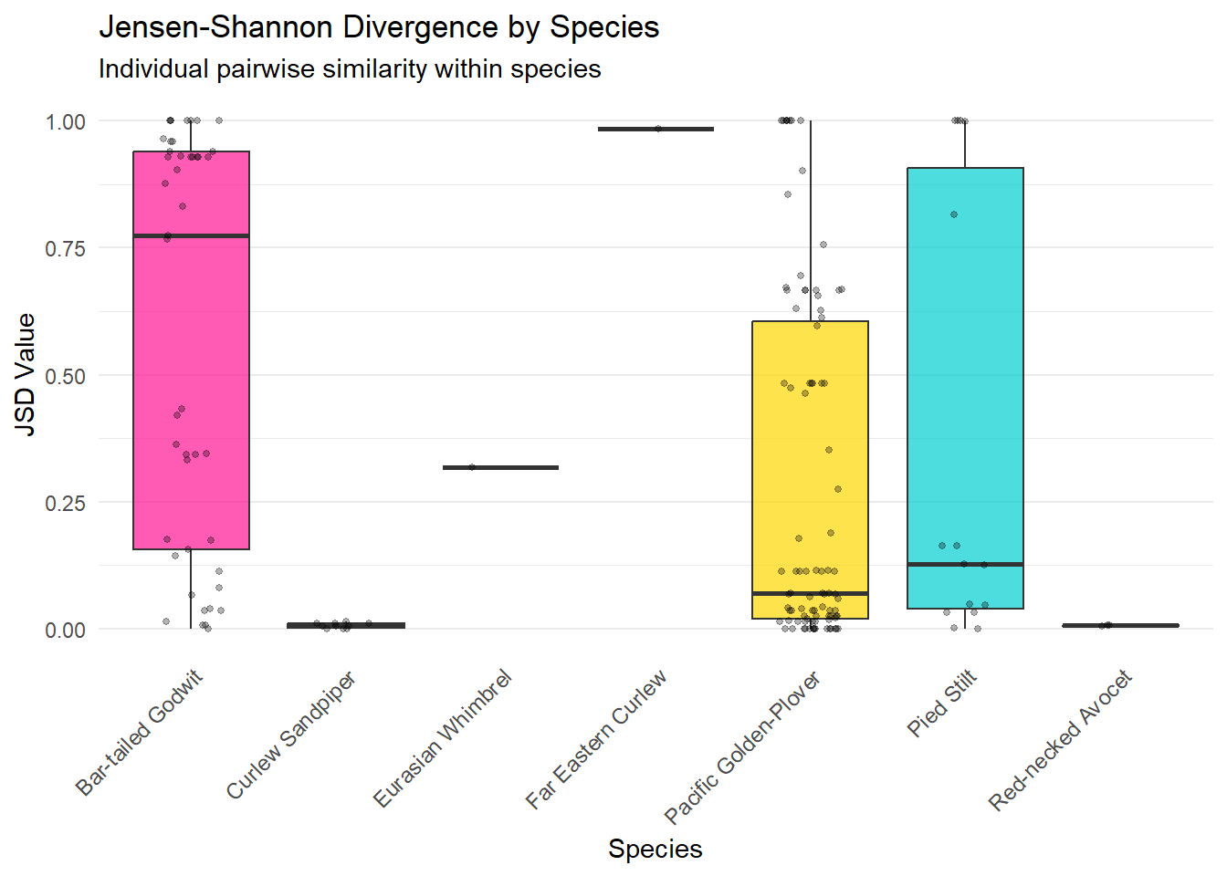
# Preparing table
jsd_results_tab <- jsd_results %>%
  filter(same_species == TRUE) %>%
  group_by(species_1) %>%
  summarise(
    n_comparisons = n(),
    mean_JSD = round(mean(JSD), 3),
    sd_JSD = round(sd(JSD), 3),
    mean_Similarity = round(mean(Similarity), 3),
    sd_Similarity = round(sd(Similarity), 3),
    .groups = "drop") %>%
  rename(speciesEN = species_1)


# Adding extra useful metrics
n_indiv <- data_all %>%
  group_by(speciesEN) %>%
  summarise(n_indiv = n_distinct(Band.ID), .groups = "drop")

# Finalise table
jsd_results_tab <- jsd_results_tab %>%
  left_join(n_indiv, by = "speciesEN") %>%
  select(speciesEN, n_indiv, everything()) %>%
arrange(mean_JSD)| Jensen-Shannon Divergence by Species | ||||||
|---|---|---|---|---|---|---|
| Individual pairwise similarity within species | ||||||
| speciesEN | n_indiv | n_comparisons | mean_JSD | sd_JSD | mean_Similarity | sd_Similarity |
| Curlew Sandpiper | 5 | 10 | 0.006 | 0.005 | 0.994 | 0.005 |
| Red-necked Avocet | 3 | 3 | 0.007 | 0.002 | 0.993 | 0.002 |
| Pacific Golden-Plover | 14 | 91 | 0.285 | 0.343 | 0.715 | 0.343 |
| Eurasian Whimbrel | 2 | 1 | 0.318 | NA | 0.682 | NA |
| Pied Stilt | 6 | 15 | 0.370 | 0.439 | 0.630 | 0.439 |
| Bar-tailed Godwit | 10 | 45 | 0.579 | 0.401 | 0.421 | 0.401 |
| Far Eastern Curlew | 2 | 1 | 0.984 | NA | 0.016 | NA |
| JSD ≈ 0 → high similarity in site composition, using same sites in same proportions. JSD ≈ 1 → low similarity in site composition, using different sets of sites or proportions. |
||||||
Species comparison | Non-Parametric test
We will use Kruskal-Wallis test if the distributions of JSD differ among species. It is a non-parametric (doesn’t assume normal distribution), it handles unequal sample sizes (different number of comparisons per species).
| Kruskal-Wallis Test Results | ||||
|---|---|---|---|---|
| Comparing value across groups | ||||
| Metric | χ2 | df | p-value | Sig. |
| Value | 39.060 | 6 | 6.967 × 10⁻⁷ | *** |
| Significance codes: *** p < 0.001, ** p < 0.01, * p < 0.05, ns = not significant (p ≥ 0.05). Green highlighting indicates significant differences. | ||||
In the aim to observe which species significantly differs from another in term of individual co;position of site used, we need to conduct pairwise test across species.
We used the Dunn method Dunn - 1964 which applies a Bonferroni correction to extract the false positive from JSD significance. The Bonferroni correction adjusts for this by dividing the significance level by the number of tests (Bonferroni -).
# If significant, do post-hoc pairwise comparisons
if(kruskal_value$p.value < 0.05) {
  dunn_jsd <- dunnTest(JSD ~ species_1,
                       data = jsd_results %>% filter(same_species == TRUE),
                       method = "bonferroni")
  print(dunn_jsd)
}| Bonferroni Correction Post-Hoc Test (Dunn) | ||||
|---|---|---|---|---|
| Pairwise JSD comparisons across species | ||||
| Comparison | Z | p unadj | p adj | Sig. |
| Bar-tailed Godwit - Curlew Sandpiper | 5.23409375 | 1.658 × 10⁻⁷ | 3.482 × 10⁻⁶ | *** |
| Bar-tailed Godwit - Eurasian Whimbrel | 0.30788506 | 7.582 × 10⁻¹ | 1.000 | ns |
| Bar-tailed Godwit - Far Eastern Curlew | -0.74359740 | 4.571 × 10⁻¹ | 1.000 | ns |
| Bar-tailed Godwit - Pacific Golden-Plover | 3.95619021 | 7.615 × 10⁻⁵ | 1.599 × 10⁻³ | ** |
| Bar-tailed Godwit - Pied Stilt | 1.37735854 | 1.684 × 10⁻¹ | 1.000 | ns |
| Bar-tailed Godwit - Red-necked Avocet | 2.96330182 | 3.044 × 10⁻³ | 6.392 × 10⁻² | ns |
| Curlew Sandpiper - Eurasian Whimbrel | -1.44789721 | 1.476 × 10⁻¹ | 1.000 | ns |
| Curlew Sandpiper - Far Eastern Curlew | -2.46152463 | 1.383 × 10⁻² | 2.905 × 10⁻¹ | ns |
| Curlew Sandpiper - Pacific Golden-Plover | -3.32847087 | 8.732 × 10⁻⁴ | 1.834 × 10⁻² | * |
| Curlew Sandpiper - Pied Stilt | -3.47632965 | 5.083 × 10⁻⁴ | 1.067 × 10⁻² | * |
| Curlew Sandpiper - Red-necked Avocet | -0.09552582 | 9.239 × 10⁻¹ | 1.000 | ns |
| Eurasian Whimbrel - Far Eastern Curlew | -0.75172622 | 4.522 × 10⁻¹ | 1.000 | ns |
| Eurasian Whimbrel - Pacific Golden-Plover | 0.40745425 | 6.837 × 10⁻¹ | 1.000 | ns |
| Eurasian Whimbrel - Pied Stilt | 0.09620662 | 9.234 × 10⁻¹ | 1.000 | ns |
| Eurasian Whimbrel - Red-necked Avocet | 1.26065985 | 2.074 × 10⁻¹ | 1.000 | ns |
| Far Eastern Curlew - Pacific Golden-Plover | 1.46476215 | 1.430 × 10⁻¹ | 1.000 | ns |
| Far Eastern Curlew - Pied Stilt | 1.12555013 | 2.604 × 10⁻¹ | 1.000 | ns |
| Far Eastern Curlew - Red-necked Avocet | 2.18133268 | 2.916 × 10⁻² | 6.123 × 10⁻¹ | ns |
| Pacific Golden-Plover - Pied Stilt | -1.11360285 | 2.654 × 10⁻¹ | 1.000 | ns |
| Pacific Golden-Plover - Red-necked Avocet | 1.78257632 | 7.466 × 10⁻² | 1.000 | ns |
| Pied Stilt - Red-necked Avocet | 2.14453471 | 3.199 × 10⁻² | 6.718 × 10⁻¹ | ns |
| Significance codes: *** p < 0.001, ** p < 0.01, * p < 0.05, ns = not significant. Green = significant. p unadj and p adj the raw and Bonferroni corrected p-values. | ||||
The table above shows which species are truly using different sites than another. Jensen-Shannon Distance measures dissimilarity in site-use composition between species pairs.
Higher JSD goes with more different site used. The Dunn test then confirms if those differences are statistically real after Bonferroni correction.
Tidal dependance | Parametric test
We now want to clarify whether birds associate site composition depending the tide, therefore likely depending their behavior (i.e., foraging vs roosting).
Applying the same method as before, we display below the JSD results depending the tide.
Important
Note: We only keep species which holds five or more individuals tagged and detected. So we can further run ANOVA analysis on the data.
Let’s display below the results of the JSD analysis in both the table and a boxplot.
| Table. Jensen-Shannon Divergence (JSD) for intra-species habitat similarity by tide state in the Hunter estuary. | |||||||||
|---|---|---|---|---|---|---|---|---|---|
| JSD ≈ 0 → high similarity in site composition, using same sites in same proportions. JSD ≈ 1 → low similarity in site composition, using different sets of sites or proportions. |
|||||||||
| Tide |
Sample Size
|
JSD (Dissimilarity)
|
Similarity (1/JSD)
|
||||||
| N indiv. | N detect. | N comp. | Mean | Median | SD | Mean | Median | SD | |
| Eurasian Whimbrel | |||||||||
| High | 2 | 15,408 | 1 | 0.310 | 0.310 | NA | 0.690 | 0.690 | NA |
| Low | 2 | 11,559 | 1 | 0.166 | 0.166 | NA | 0.834 | 0.834 | NA |
| Curlew Sandpiper | |||||||||
| High | 5 | 374,495 | 10 | 0.003 | 0.005 | 0.003 | 0.997 | 0.995 | 0.003 |
| Low | 5 | 294,779 | 10 | 0.006 | 0.000 | 0.008 | 0.994 | 1.000 | 0.008 |
| Red-necked Avocet | |||||||||
| High | 3 | 83,598 | 3 | 0.007 | 0.006 | 0.005 | 0.993 | 0.994 | 0.005 |
| Low | 3 | 26,612 | 3 | 0.063 | 0.063 | 0.044 | 0.937 | 0.937 | 0.044 |
| Pacific Golden-Plover | |||||||||
| High | 14 | 657,498 | 91 | 0.308 | 0.114 | 0.334 | 0.692 | 0.886 | 0.334 |
| Low | 14 | 668,764 | 91 | 0.288 | 0.052 | 0.345 | 0.712 | 0.948 | 0.345 |
| Pied Stilt | |||||||||
| High | 6 | 492,414 | 15 | 0.368 | 0.100 | 0.440 | 0.632 | 0.900 | 0.440 |
| Low | 6 | 391,507 | 15 | 0.379 | 0.216 | 0.437 | 0.621 | 0.784 | 0.437 |
| Bar-tailed Godwit | |||||||||
| High | 9 | 115,486 | 36 | 0.531 | 0.557 | 0.413 | 0.469 | 0.443 | 0.413 |
| Low | 9 | 25,522 | 36 | 0.580 | 0.575 | 0.362 | 0.420 | 0.425 | 0.362 |
| High | 2 | 21,392 | 1 | 0.984 | 0.984 | NA | 0.016 | 0.016 | NA |
| Low | 2 | 51,535 | 1 | 0.984 | 0.984 | NA | 0.016 | 0.016 | NA |
| Legend. n_indiv: tagged individuals per species×tide combination; n_detect: total number of detections per species×tide combination; n_comparisons: pairwise comparisons; mean_JSD ± sd_JSD: average dissimilarity in site used; mean_Similarity ± sd_Similarity: 1/JSD (average site used similarity). Low tide rows blue, High tide rows yellow. | |||||||||
jsd_for_plot_tide %>%
  filter(metric == "JSD") %>%
  ggplot(aes(x     = species_1,
             y     = value,
             fill  = species_1,
             alpha = tideHighLow,
             group = interaction(species_1, tideHighLow))) +

  geom_boxplot(position      = position_dodge(width = 0.8),
               outlier.shape = 16,
               outlier.size  = 1.5) +

  geom_point(position = position_jitterdodge(jitter.width = 0.15,
                                             dodge.width  = 0.8),
             size = 1.1) +

  scale_fill_manual(values = species_colors) +
  scale_alpha_manual(values = c("High" = 1.0, "Low" = 0.35)) +

  labs(
    title    = "Within-species Jensen-Shannon Divergence by Tide",
    subtitle = "Pairwise JSD between individuals — High tide (solid) vs Low tide (transparent)",
    x        = NULL,
    y        = "Jensen-Shannon Divergence") +

  theme_minimal() +
  theme(
    legend.position    = "none",
    axis.text.x        = element_text(angle = 45, hjust = 1, size = 9),
    panel.grid.major.x = element_blank(),
    plot.title         = element_text(face = "bold"),
    plot.subtitle      = element_text(size = 9, color = "grey40"))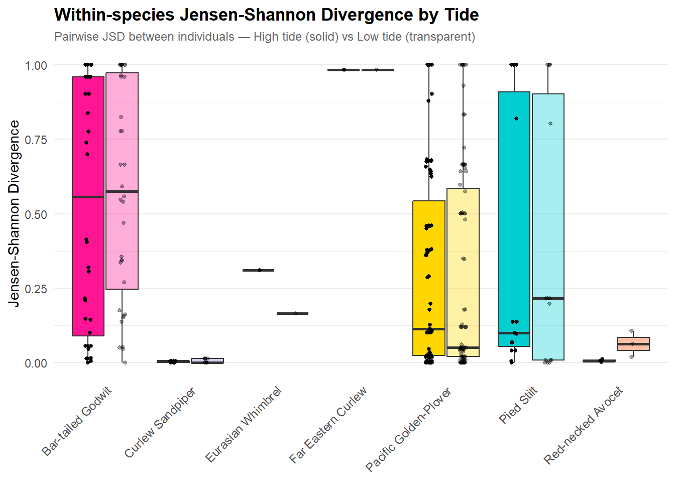
We now want to test whether JSD values are different across individual of a same species at High and Low tides.
To do so, we will conduct a two-paired ANOVA analysis, therefore we must verify data normality and homogeneity first.
results_jsd_tide<- data.frame()
assumptions_jsd <- data.frame()

for (sp in species_list_jsd) {

  df <- subset(jsd_for_plot_tide, species_1 == sp & metric == "JSD")
  df <- na.omit(df)
  df$Band.ID_1   <- droplevels(df$Band.ID_1)
  df$Band.ID_2   <- droplevels(df$Band.ID_2)
  df$tideHighLow <- droplevels(df$tideHighLow)

  # Check levels before fitting
  n_tide <- nlevels(df$tideHighLow)
  n_id   <- nlevels(df$Band.ID_1)

  # Skip species with insufficient variation to fit any model
  if (n_id < 2) {
    message("Skipping ", sp, ": fewer than 2 individuals")
    next
  }

  # Build formula depending on whether tide has 2 levels
  model_formula <- if (n_tide >= 2) {
    value ~ Band.ID_1 + tideHighLow
  } else {
    message("Note: ", sp, " has only 1 tide level — fitting without tideHighLow")
    value ~ Band.ID_1
  }

  model <- aov(model_formula, data = df)
  s     <- summary(model)[[1]]

  # --- ANOVA results ---
  # Only loop over terms that were actually in the model
  terms_to_check <- intersect(c("Band.ID_1", "tideHighLow"), rownames(s))

  for (term in terms_to_check) {
    results_jsd_tide <- rbind(results_jsd_tide, data.frame(
      Species = sp,
      Metric  = "JSD",
      Term    = ifelse(term == "tideHighLow", "Tide effect",
                ifelse(term == "Band.ID_1",   "Individual", term)),
      Df      = s[term, "Df"],
      SS      = round(s[term, "Sum Sq"],  4),
      MS      = round(s[term, "Mean Sq"], 4),
      F_value = round(s[term, "F value"], 3),
      p_value = round(s[term, "Pr(>F)"],  4),
      stringsAsFactors = FALSE
    ))
  }

  # --- Normality (Shapiro-Wilk on residuals) ---
  sw <- shapiro.test(residuals(model))

  # --- Homogeneity of variance (Levene's test — only if tide has >= 2 levels) ---
  lev <- if (n_tide >= 2) {
    tryCatch(
      leveneTest(value ~ tideHighLow, data = df, center = median),
      error = function(e) NULL
    )
  } else {
    NULL
  }

  assumptions_jsd <- rbind(assumptions_jsd, data.frame(
    Species      = sp,
    Metric       = "JSD",
    N            = nrow(df),
    Independence = "By design",
    SW_W         = round(sw$statistic,  4),
    SW_p         = round(sw$p.value,    4),
    Normality    = ifelse(sw$p.value > 0.05, "✓ Met", "✗ Violated"),
    Levene_F     = ifelse(!is.null(lev), round(lev[1, "F value"], 4), NA),
    Levene_p     = ifelse(!is.null(lev), round(lev[1, "Pr(>F)"],  4), NA),
    Homogeneity  = ifelse(!is.null(lev),
                     ifelse(lev[1, "Pr(>F)"] > 0.05, "✓ Met", "✗ Violated"),
                     "Insufficient levels"),
    stringsAsFactors = FALSE
  ))
}| ANOVA Assumption Tests — JSD | ||||||||
|---|---|---|---|---|---|---|---|---|
| Normality (Shapiro-Wilk) and Homogeneity of Variance (Levene’s test) | ||||||||
| Metric | n | Independence |
Shapiro-Wilk
|
Levene's Test
|
||||
| W | p value | Normality | F | p value | Homogeneity | |||
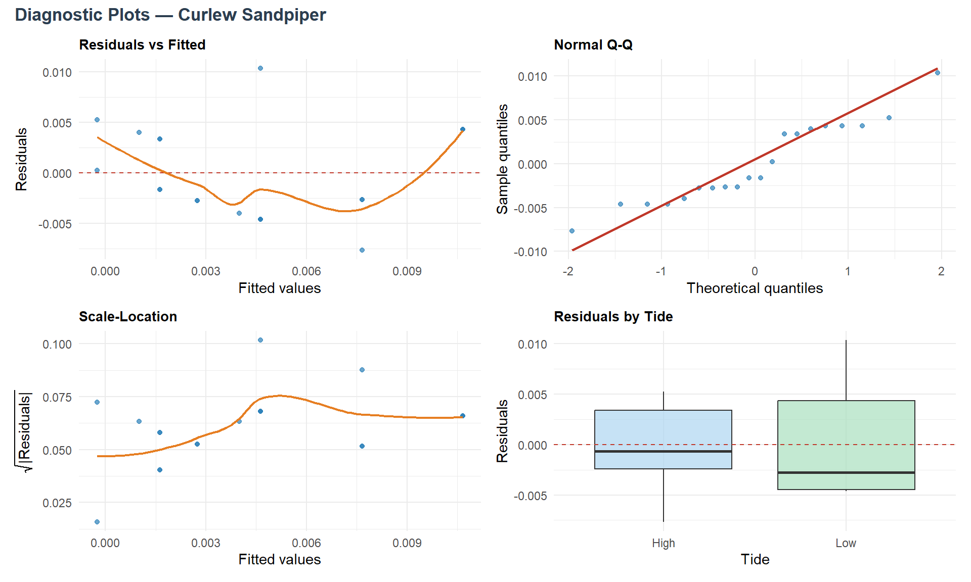
| Curlew Sandpiper | ||||||||
| JSD | 20 | By design | 0.9275 | 0.1383 | ✓ Met | 2.4000 | 0.1387 | ✓ Met |
| Pacific Golden-Plover | ||||||||
| JSD | 182 | By design | 0.8438 | 0.0000 | ✗ Violated | 0.0646 | 0.7996 | ✓ Met |
| Bar-tailed Godwit | ||||||||
| JSD | 72 | By design | 0.9711 | 0.0959 | ✓ Met | 4.4789 | 0.0379 | ✗ Violated |
| Pied Stilt | ||||||||
| JSD | 30 | By design | 0.9479 | 0.1484 | ✓ Met | 0.0136 | 0.9081 | ✓ Met |
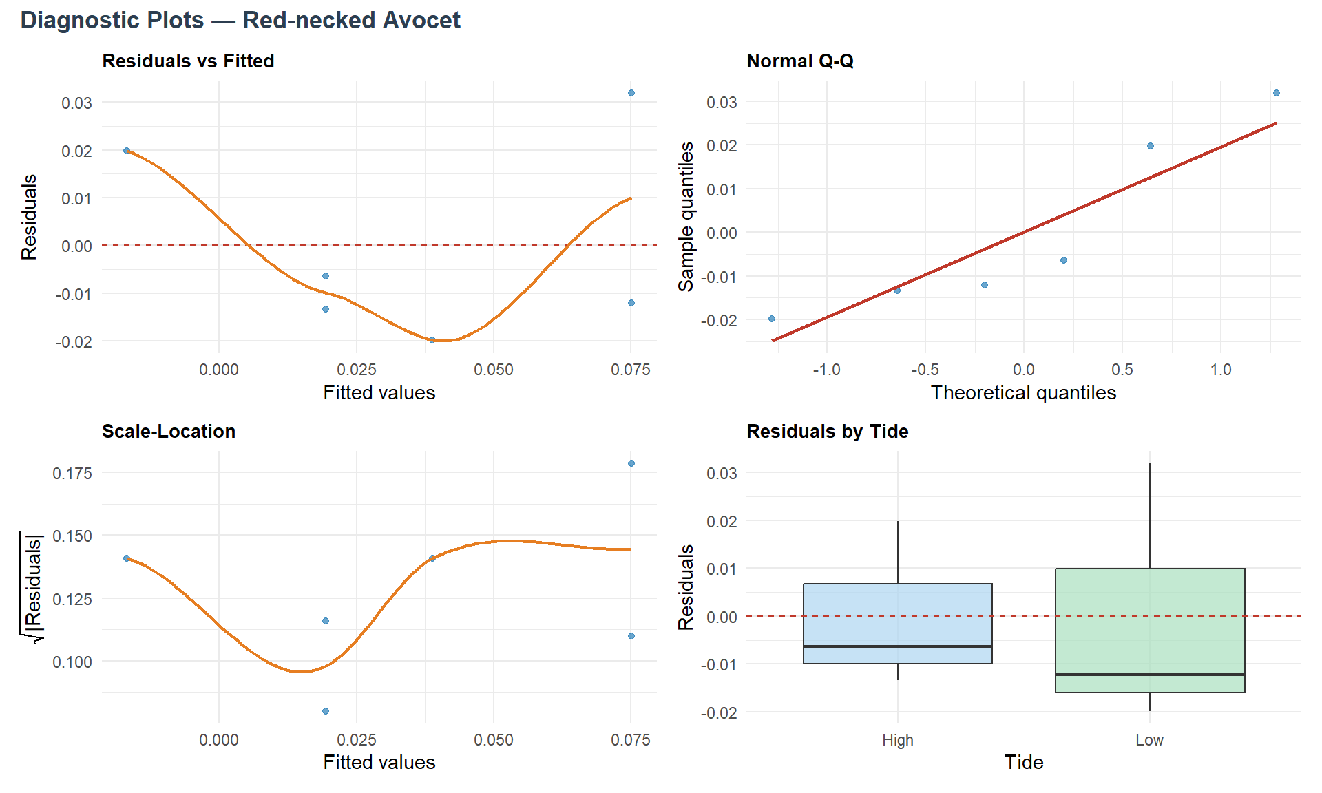
| Red-necked Avocet | ||||||||
| JSD | 6 | By design | 0.8553 | 0.1737 | ✓ Met | 3.0836 | 0.1539 | ✓ Met |
| Independence: verified by design — each Band.ID is a unique individual measured once per tide condition. Shapiro-Wilk: H₀ = residuals are normally distributed; p > 0.05 → assumption met. Levene’s test: H₀ = variances are equal across tide groups; p > 0.05 → assumption met. |
||||||||
Below are displayed Res. vs. Fitted, Normal Q-Q, Scale-Location and Res. by tide plots, for each species.


Now ANOVA assumptions are verified, let’s see the ANOVA analysis results.
results_jsd_tide <- results_jsd_tide %>%
  mutate(
    sig = case_when(
      p_value < 0.001 ~ "***",
      p_value < 0.01  ~ "**",
      p_value < 0.05  ~ "*",
      p_value < 0.1   ~ ".",
      TRUE            ~ ""
    )
  )

# ── ANOVA table ──────────────────────────────────────────────────────────────

results_jsd_tide %>%
  gt(groupname_col = "Species", rowname_col = "Term") %>%

  tab_header(
    title    = md("**Two-Way ANOVA Results — JSD**"),
    subtitle = md("*value ~ Band.ID + tideHighLow — by Species*")
  ) %>%

  cols_label(
    Metric  = "Metric",
    Df      = "df",
    SS      = "Sum Sq",
    MS      = "Mean Sq",
    F_value = "F value",
    p_value = "p value",
    sig     = ""
  ) %>%

  tab_style(
    style     = cell_text(color = "#c0392b", weight = "bold"),
    locations = cells_body(
      columns = vars(p_value, sig),
      rows    = sig %in% c("*", "**", "***", ".")
    )
  ) %>%

  opt_row_striping() %>%

  tab_source_note(
    source_note = "Significance codes: *** p<0.001  ** p<0.01  * p<0.05  . p<0.1"
  ) %>%

  tab_options(
    row_group.font.weight      = "bold",
    row_group.background.color = "#f0f4f8",
    heading.align              = "left",
    table.font.size            = 13
)| Two-Way ANOVA Results — JSD | |||||||
|---|---|---|---|---|---|---|---|
| value ~ Band.ID + tideHighLow — by Species | |||||||
| Metric | df | Sum Sq | Mean Sq | F value | p value | ||
| Curlew Sandpiper | |||||||
| Tide effect | JSD | 1 | 0.0000 | 0.0000 | 1.671 | 0.2157 | |
| Pacific Golden-Plover | |||||||
| Tide effect | JSD | 1 | 0.0177 | 0.0177 | 0.199 | 0.6563 | |
| Bar-tailed Godwit | |||||||
| Tide effect | JSD | 1 | 0.0435 | 0.0435 | 0.406 | 0.5266 | |
| Pied Stilt | |||||||
| Tide effect | JSD | 1 | 0.0009 | 0.0009 | 0.150 | 0.7018 | |
| Red-necked Avocet | |||||||
| Tide effect | JSD | 1 | 0.0046 | 0.0046 | 6.418 | 0.0852 | . |
| Significance codes: *** p<0.001 ** p<0.01 * p<0.05 . p<0.1 | |||||||