library(motus)
library(dplyr)
library(here)
library(forcats)
library(ggplot2)
library(lubridate)
library(tidyr)
library(purrr)
library(readr)
library(bioRad)
library(hms)
library(dplyr)
library(ggplot2)
library(scales)
library(gt)Station usage - hours
Load your data in your R environment - see Load & Format > Reproducibility
And load your activity table too!
recv.act <- tbl(sql.motus, "activity")  %>%
  collect() %>%
  as.data.frame() %>%
  rename(deviceID = "motusDeviceID") %>%
  # keep our deployed antennas only
  filter(deviceID %in% unique(recv$deviceID)) %>%
  # Set the time properly - IMPORTANT
  mutate(date = as_datetime(as.POSIXct(hourBin* 3600,
                                       origin = "1970-01-06",
                                       tz = "UTC")),
         dateAus = as_datetime(as.POSIXct(hourBin* 3600,
                                          origin = "1970-01-06",
                                          tz = "UTC"),
                               tz = "Australia/Sydney"))
Pre-requisite
This analysis compares the time available for each tidal category (Diurnal High Tide, Nocturnal High Tide, Diurnal Low Tide and Nocturnal Low tide) with the time each shorebird species spent at Motus stations.
First, we need to determine the available time for each species group and for each Motus station. Second, we need to calculate the time used for each bird in every species and for each MOTUS stations too.
The below procedure breaks down how we assessed:
- Tide variable
- The time available
- The time used
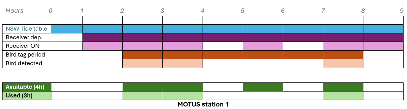
Schema: Definition of available and used periods across bird individuals and Motus stations
TIDE VARIABLE
Based on New South Wales Tide Tables we were able to extract and classify the total time for each of the four categories of tide that occurred within the Hunter estuary. Note that one data-set is provided at the estuary scale, therefore, we assume the tide is occurring at the same scale, time, frequency and amplitude across our MOTUS stations.
Tide table informs for Low and High tide peaks. Half of the period between peak n and peak n-1 is taken, added to the period between peak n and peak n+1, then expanded in hours for further analysis. The tide associated to peak n defines its variable period (i.e. red lines below is defined as high tide since peak n is a high tide peak).
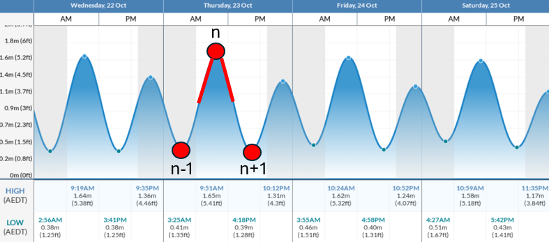
Schema: Definition of tide variables (high or low) for one period (red line)
tide_data <- tide_data %>%

  arrange(tideDateTimeAus) %>%
  mutate(prev_time = lag(tideDateTimeAus),
         next_time = lead(tideDateTimeAus) ) %>%
  filter(!is.na(prev_time) & !is.na(next_time)) %>%

  # Get the duration of the tide centered around Peak 2 (P2), with start halfway between P1 and P2, and with end btw P2-P3
  mutate(duration_h = as.numeric(difftime(tideDateTimeAus, prev_time, units = "hours")/2 +
                                    difftime(next_time, tideDateTimeAus, units = "hours")/2)) %>%

  # Rename for consistency
  rename(tideHighLow = high_low,
         timeAus = tideDateTimeAus,
         tideDiel = day_night) %>%
  select(timeAus, tideCategory, tideHighLow, tideDiel, duration_h, sunriseNewc, sunsetNewc) %>%

  # Factorise
  mutate(tideCategory = as_factor(tideCategory))
TIME AVAILABLE
Now tide data ready to be processed, we need to define for each individual (birds) and across each Motus stations, what was the amount of time available for the four tide categories.
Available time for each Motus stations is accessed with activity table: each row is a dated record of noise or a tag detected - see Survey effort > Activity table.
We need to extract the temporal coverage of each station, starting from deployment date to the last recorded activity, and expand this period in hours.
# Sort the terminated serno (if terminated, ie. one box removed from one antenna site, a date comes along)
# but still needed for accessing survey effort as the station is currently running with another serno
recv.act.term <- recv.act %>%
  left_join(recv %>%
              filter(!is.na(timeEndAus)) %>%
              select(deviceID, serno, recvDeployName),
            "deviceID") %>%
  filter(!is.na(recvDeployName)) %>%
  mutate(SernoStation = paste0(recvDeployName, "_", serno))

# Sort the currently running serno
recv.act.runn <- recv.act %>%
  left_join(recv %>%
              filter(is.na(timeEndAus)) %>%
              select(deviceID, serno, recvDeployName),
            "deviceID") %>%
  filter(!is.na(recvDeployName)) %>%
  mutate(SernoStation = paste0(recvDeployName, "_", serno))

# Merging in one data-set to use Station's name further + pick-up the rounded hours
recv.act <- bind_rows(recv.act.runn, recv.act.term) %>%
  mutate(hour_dt = round_date(dateAus, "hour"))

# Providing helpful variables
recv <- recv %>%
  mutate(SernoStation = paste0(recvDeployName, "_", serno),
         lisStart = timeStartAus,
         lisEnd = if_else(
           is.na(timeEndAus), # means the station is still running since the last data downloading
           with_tz(Sys.time(), "Australia/Sydney"),
           with_tz(as_datetime(timeEndAus, tz = "UTC"), "Australia/Sydney")) )

# Generating hourly sequences per SernoStation from start to end dates of the deviceID at particular sites
recv_hours <- recv %>%
  select(recvDeployName, deviceID, SernoStation, lisStart, lisEnd) %>%
  group_by(SernoStation) %>%
  rowwise() %>%
  mutate(hour_dt = list(seq(from = round_date(lisStart, unit = "hour"),
                            to = round_date(lisEnd, unit = "hour"),
                            by = "hour")) ) %>%
  unnest(cols = c(hour_dt)) %>%
  ungroup()

# Simplify station variables (recvDeployName)
recv <- recv %>%
  select(!recvDeployName)
recv$recvDeployName <- sub("_SG-.*", "", recv$SernoStation)

recv_hours <- recv_hours %>%
  select(!recvDeployName)
recv_hours$recvDeployName <- sub("_SG-.*", "", recv_hours$SernoStation)
We now how the complete temporal coverage, expanded in hours, for each Motus station.
However, due to some temporary failures or maintenance (see Survey effort > Operational periods), the actual period a station was operational may be different than the complete temporal coverage. So, we must determine when a station was not operational and substract these off-hours to the complete temporal coverage.
# Distinguish station from mixed recv + Giving operational variable (= TRUE when existing values from act table)
recv_hours <- recv_hours %>%
  left_join(recv.act %>%
              distinct(recvDeployName, hour_dt) %>%
              mutate(operational = TRUE),
            by = c("recvDeployName", "hour_dt")) %>%
  mutate(operational = if_else(is.na(operational), FALSE, TRUE))

# /!\ Due to unknown error? Have to set this manually
recv_hours <- recv_hours %>%
  mutate(operational = case_when(
    recvDeployName == "Fullerton Entrance" &
      hour_dt > as.POSIXct("2023-04-02") &
      hour_dt < as.POSIXct("2023-04-05") ~ FALSE,
    TRUE ~ operational))

# Summary table
off_runs <- recv_hours %>%
  arrange(recvDeployName, hour_dt) %>%
  group_by(recvDeployName) %>%
  mutate(off_run_id = consecutive_id(operational == FALSE)) %>%
  ungroup() %>%

  filter(operational == FALSE) %>%

  group_by(recvDeployName, off_run_id) %>%
  summarise(
    start_off = min(hour_dt),
    end_off = max(hour_dt),
    tot_off_hours = n(),
    .groups = "drop") %>%

  filter(tot_off_hours > 24)

# Unique recvDeployNames from off_runs
recv_names <- unique(recv_hours$recvDeployName)

# Split tide_data into a named list with one element per recvDeployName
tide_data_list <- setNames(vector("list", length(recv_names)), recv_names)

for(name in recv_names) {
  # Get off intervals for this recvDeployName
  intervals <- off_runs %>%
    filter(recvDeployName == name) %>%
    select(start_off, end_off)

  # Get deployment start and end dates for this recvDeployName
  deploy <- recv_hours %>%
    filter(recvDeployName == name) %>%
    summarise(
      lisStart = min(lisStart, na.rm = TRUE),
      lisEnd = max(lisEnd, na.rm = TRUE)
    )

  # Filter tide_data by deployment period
  td <- tide_data %>%
    filter(timeAus >= deploy$lisStart & timeAus <= deploy$lisEnd) %>%
    mutate(recvDeployName = name)

  if(nrow(intervals) > 0) {
    # Vectorized exclusion of off intervals
    is_in_off <- sapply(td$timeAus, function(t) {
      any(t >= intervals$start_off & t <= intervals$end_off)
    })
    td <- td[!is_in_off, ]
  }
  tide_data_list[[name]] <- td
}

tide_data_df <- bind_rows(tide_data_list) %>%
  mutate(hour_dt = round_date(timeAus, unit = "hour"))            # AVAILABLE TIME (tide categories covering same time as recv survey effort)

# Finalise data set for receiver ON with tidal data, per hour
total_recv_tide_data <- tide_data_df %>%
  group_by(recvDeployName) %>%

  # Expand per hour bin
  summarise(hour_seq = list(seq(min(hour_dt), max(hour_dt), by = "hour")), .groups = "drop") %>%
  unnest(hour_seq) %>%
  rename(hour_dt = hour_seq) %>%

  # Match tide data to hourly grid
  # Hours WITHOUT tide data get NA values across all columns but we'll deal with this later
  left_join(tide_data_df, by = c("recvDeployName", "hour_dt"))
Temporal coverage for each station is now reduced to its operational periods, and ready to be processed.
We now assign each bird its own available time period, spanning from its tagging date to its last Motus detection, and expanded to hourly resolution too.
# Get the monitored period of each bird
period_sp <- data_all  %>%
  group_by(Band.ID) %>%
  reframe(DateAUS.Trap = first(DateAUS.Trap),
          last_dateAus = max(dateAus),
          speciesEN = speciesEN) %>%
  unique()

# Expand one row per hours to each individual across its whole period (this is the available time)
bird_hours <- period_sp %>%
  group_by(Band.ID) %>%
  rowwise() %>%
  mutate(hour_dt = list(seq(from = as.POSIXct(ymd(DateAUS.Trap), tz = "UTC"),
                            to = as.POSIXct(last_dateAus, tz = "UTC"),
                            by = "hour"))) %>%
  unnest(cols = c(hour_dt)) %>%
  ungroup()

# Duplicate in as many list as many stations
recv_names <- unique(recv_hours$recvDeployName)
bird_data_list <- setNames(vector("list", length(recv_names)), recv_names)

for(name in recv_names) {

  valid_hours_recv <- total_recv_tide_data %>%
    filter(recvDeployName == name) %>%
    pull(hour_dt)

  valid_hours_bird_recv <- bird_hours %>%
    filter(hour_dt %in% valid_hours_recv)

  valid_hours_bird_recv$name <- name


  bird_data_list[[name]] <- valid_hours_bird_recv
}

# ADD TIDE TO AVAILABLE TIME
# The NA cols left over before from recv table, now also filtered out based on available time coming from bird periods table
get.tideIndex <- function(time){return(which.min(abs(tide_data$timeAus - time)))}

available_bird_recv_time <- bind_rows(bird_data_list) %>%
  mutate(hour_dt = force_tz(hour_dt, "Australia/Sydney")) %>%
  # Remove rows with ANY NA
  filter(if_all(everything(), ~ !is.na(.))) %>%
  mutate(tideIndex = map_dbl(hour_dt, get.tideIndex))

# Extract tide categories thanks to tide index (row order in available_bird_recv_time)
tide_values <- tide_data[available_bird_recv_time$tideIndex, c("tideCategory")]

# Merge tide categories to available_bird_recv_time and factorise the variables
available_bird_recv_time <- available_bird_recv_time %>%
  mutate(tideCategory = as_factor(tide_values$tideCategory))

# FINALISE AVAILABLE TIME
available_bird_recv_time <- available_bird_recv_time %>%
  rename(recvDeployName = name) %>%
  group_by(Band.ID, speciesEN, recvDeployName, tideCategory)  %>%
  summarise(duration_h = n()) %>%
  mutate(tideDiel = if_else(grepl("Diurnal", tideCategory), "Diurnal", "Nocturnal"),
         tideHighLow = if_else(grepl("High", tideCategory), "High", "Low")) %>%
  select(Band.ID, speciesEN, recvDeployName, tideCategory, tideDiel, tideHighLow, duration_h)
The available time is now defined for each bird across each Motus station, taking into account the periods where stations where ON only. The available periods are expanded in hours and the tide condition is associated.
TIME USED
Let’s now determine the time used for each bird for each Motus station.
The time used is defined by multiplying the number of detections (meaning the number of rows) by the duration of a pulse (pulse interval). We assume that if an individual is detected by a receiver once, the individual was at least in the station coverage for the duration of the signal pulse. Duration differ depending tag models - see table below.
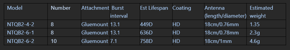
Pulse Interval depending Lotek nanotag models
# USED TIME (amount of time each bird spent during each category of tide and at each station)
# Provide the burst interval value depending Lotek-nano tag model (scd)
data_bird <- data_all %>%
  mutate(burst_inter = ifelse(tagModel == "NTQB2-6-2", dseconds(7.1), dseconds(13.1))) %>%
  select(timeAus, sunriseNewc, sunsetNewc, tideCategory, tideHighLow, tideDiel,
         speciesEN, tagModel, recvDeployName, recv,speciesSci, Band.ID, burst_inter)

used_bird_recv_time <- data_bird %>%
  group_by(Band.ID, speciesEN, recvDeployName, tideCategory)  %>%
  summarise(duration_sec = sum(burst_inter)) %>%
  mutate(duration_h = round(duration_sec / 3600, 0),
         tideDiel = if_else(grepl("Diurnal", tideCategory), "Diurnal", "Nocturnal"),
         tideHighLow = if_else(grepl("High", tideCategory), "High", "Low")) %>%
  select(Band.ID, speciesEN, recvDeployName, tideCategory, tideDiel, tideHighLow, duration_h)
Usage rate
Now that the used and available time have been determined for each individual and for each Motus station, we can relate these two elements together with the Usage rate (or rate of use).
\[ \text{Usage rate} = \frac{\text{Time used}}{\text{Time available}} \times 100 \quad \textit{across stations and species} \]
Some cases may happen where the time used was over the available. It may occur because multiplying each bird detection by its pulse interval duration overestimates the actual time used. For example, if a bird is detected twice with a 13-second pulse interval—once at second 1 and again at second 14—this results in 2 detections over 14 seconds. However, simply multiplying the detections by the pulse interval (2 × 13 seconds) incorrectly estimates the total time used as 26 seconds.
| Band.ID | speciesEN | recvDeployName | tideCategory | tideDiel | tideHighLow | available_t | used_t | rate_use |
|---|---|---|---|---|---|---|---|---|
| 6318617 | Pacific Golden-Plover | Curlew Point | Diurnal_Low | Diurnal | Low | 346 | 351 | 101.4451 |
| 6318617 | Pacific Golden-Plover | Curlew Point | Diurnal_High | Diurnal | High | 437 | 461 | 105.4920 |
| 7176824 | Bar-tailed Godwit | Curlew Point | Nocturnal_High | Nocturnal | High | 6 | 8 | 133.3333 |
| 7176824 | Bar-tailed Godwit | Tomago | Nocturnal_High | Nocturnal | High | 6 | 9 | 150.0000 |
| 7394027 | Bar-tailed Godwit | Tomago | Nocturnal_High | Nocturnal | High | 49 | 52 | 106.1224 |
| 7394040 | Bar-tailed Godwit | Curlew Point | Diurnal_High | Diurnal | High | 6 | 8 | 133.3333 |
| 7394040 | Bar-tailed Godwit | Curlew Point | Nocturnal_Low | Nocturnal | Low | 6 | 13 | 216.6667 |
Note: We decided to force n = 5 out of 1512 cases where the rate used was between 100 and 140 % to equal 100 %.
And we decided to remove n = 2 cases where the rate used was over 140 %, considering the tag might simply have fell of the bird within the vicinity of the station.
Reminder: one case is made of the combination from an individual recorded at a Motus station for a specific tide condition. - See table above.
figure_plot <- figure_plot %>%

  mutate(rate_use = ifelse(rate_use > 100 & rate_use < 140, 100, rate_use)) %>% # force 100-140 rate values to equal 100 %
  mutate(rate_use = ifelse(rate_use >= 140, NA, rate_use)) %>%                  # remove rates above 140 %

  mutate(speciesType = factor(shorebird_class[speciesEN],
                               levels = c("migratory", "resident"))) %>%

  filter(!speciesEN %in% c("Masked Lapwing"))
Note: We filtered out Masked Lapwing from the analysis, since they have too few data.
Now, everything is ready to format the data for plot and to visualise the results for Usage rate and Hourly usage across the Motus stations of our local array.
# Track size sample
counts <- used_bird_recv_time %>%
      group_by(speciesEN) %>%
      summarise(n = n_distinct(Band.ID)) %>%
      mutate(label = paste0(speciesEN, " (n = ", n, ")"))
label_vec <- setNames(counts$label, counts$speciesEN)
# Tide and species groupings
tide_levels <- c("Low", "High")
species_types <- unique(shorebird_class)
# Simplified function - no min_n_nonzero check
make_plot <- function(tide_level, species_type) {
data_sub <- figure_plot %>%
filter(tideHighLow == tide_level) %>%
mutate(species_class = shorebird_class[speciesEN]) %>%
filter(species_class == species_type)
p <- ggplot(data_sub,
aes(x = factor(recvDeployName, levels = sort(unique(recvDeployName))),
y = rate_use,
fill = tideDiel))
# Always add boxplot for all available data
p <- p +
geom_boxplot(outlier.shape = NA,
varwidth = FALSE,
position = position_dodge(width = 0.8, preserve = "single")) +
# Always show individual points
geom_point(aes(shape = tideDiel),
position = position_dodge(width = 0.8),
alpha = 1, size = 1.5,
show.legend = FALSE) +
scale_shape_manual(values = c("Diurnal" = 21, "Nocturnal" = 16)) +
facet_wrap(~ speciesEN,
labeller = labeller(speciesEN = label_vec)) +
labs(x = "Receiver Deployment",
y = "Rate of Use (%)",
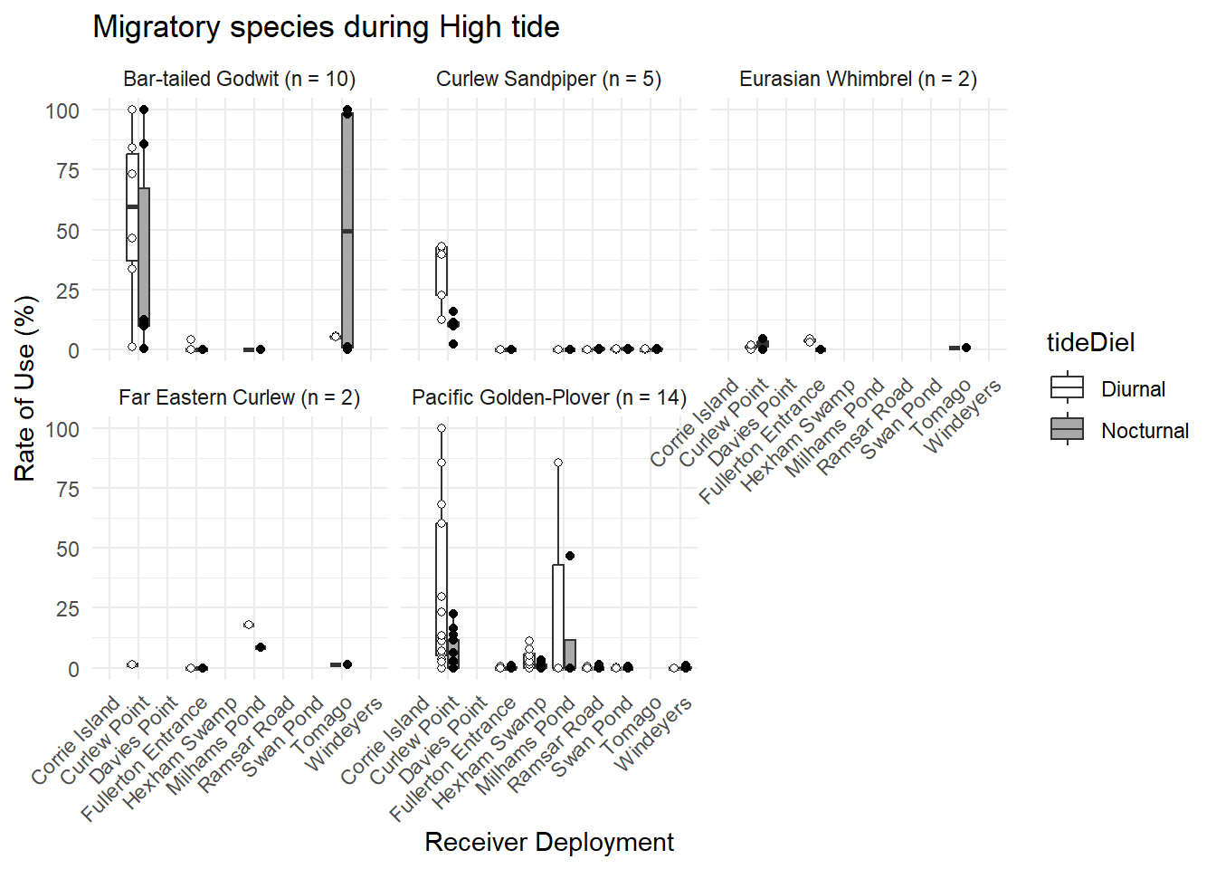
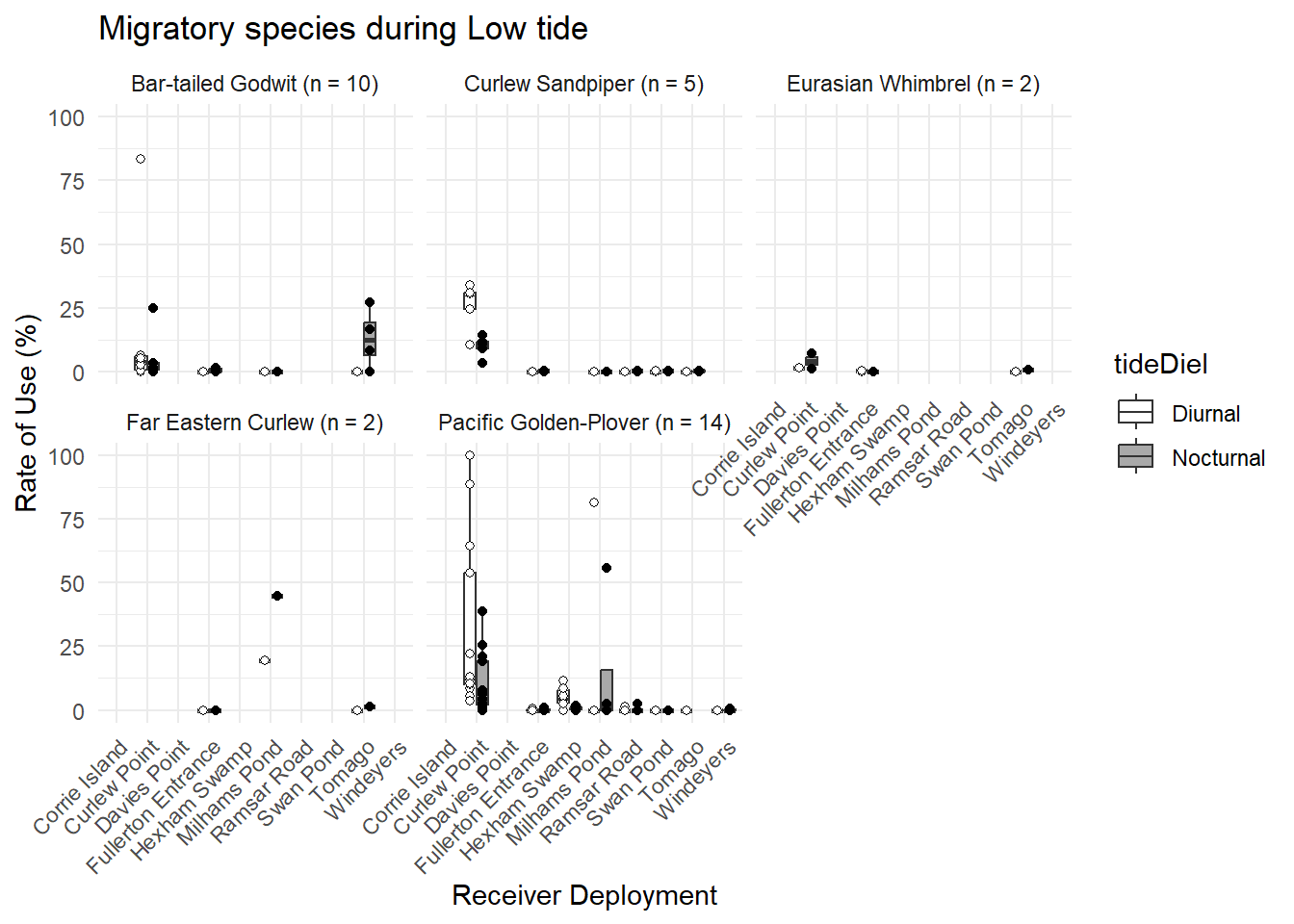
title = paste(ifelse(species_type == "migratory",
"Migratory species", "Resident species"),
"during", tide_level, "tide")) +
coord_cartesian(ylim = c(0, 100)) +
theme_minimal() +
scale_fill_manual(values = c("Diurnal" = "white", "Nocturnal" = "darkgrey")) +
theme(axis.text.x = element_text(angle = 45, hjust = 1))
return(p)
}
# Generate all plots
plots_used_rate <- cross2(tide_levels, species_types) %>%
purrr::map(~ make_plot(.x[[1]], .x[[2]]))# General function to provide one table with stats values
make_summary_table <- function(tide_level, species_type) {
data_sub <- figure_plot %>%
filter(tideHighLow == tide_level) %>%
mutate(species_class = shorebird_class[speciesEN]) %>%
filter(species_class == species_type)
summary_table <- data_sub %>%
group_by(speciesEN, recvDeployName, tideDiel) %>%
summarise(
n_individual = n(),
min = round(min(rate_use, na.rm = TRUE), 1),
q1 = round(quantile(rate_use, 0.25, na.rm = TRUE),1),
median = round(median(rate_use, na.rm = TRUE),1),
q3 = round(quantile(rate_use, 0.75, na.rm = TRUE),1),
max = round(max(rate_use, na.rm = TRUE),1),
mean = round(mean(rate_use, na.rm = TRUE),1),
sd = round(sd(rate_use, na.rm = TRUE),1),
.groups = 'drop'
) %>%
arrange(speciesEN, recvDeployName, tideDiel) %>%
rename(Species = "speciesEN", Station = "recvDeployName", condition = "tideDiel")
return(summary_table)
}
# One table per conditions
high_migratory <- make_summary_table("High", "migratory")
high_resident <- make_summary_table("High", "resident")
low_migratory <- make_summary_table("Low", "migratory")
low_resident <- make_summary_table("Low", "resident")RESIDENT BIRDS
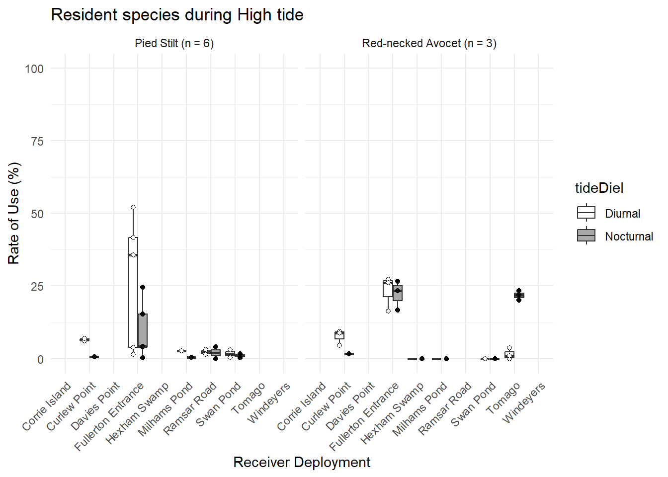
High Tide Resident birds
| Statistics - High Tide Resident Species | ||||||||||
|---|---|---|---|---|---|---|---|---|---|---|
| Species | Station | condition | n_individual | min | q1 | median | q3 | max | mean | sd |
| Pied Stilt | Corrie Island | Diurnal | 3 | Inf | NA | NA | NA | -Inf | NaN | NA |
| Pied Stilt | Corrie Island | Nocturnal | 3 | Inf | NA | NA | NA | -Inf | NaN | NA |
| Pied Stilt | Curlew Point | Diurnal | 4 | 6.1 | 6.3 | 6.5 | 6.7 | 6.9 | 6.5 | 0.6 |
| Pied Stilt | Curlew Point | Nocturnal | 4 | 0.5 | 0.5 | 0.5 | 0.5 | 0.5 | 0.5 | NA |
| Pied Stilt | Davies Point | Diurnal | 3 | Inf | NA | NA | NA | -Inf | NaN | NA |
| Pied Stilt | Davies Point | Nocturnal | 3 | Inf | NA | NA | NA | -Inf | NaN | NA |
| Pied Stilt | Fullerton Entrance | Diurnal | 6 | 1.5 | 3.8 | 35.7 | 41.7 | 52.1 | 27.0 | 23.0 |
| Pied Stilt | Fullerton Entrance | Nocturnal | 6 | 0.3 | 4.0 | 4.1 | 15.4 | 24.6 | 9.7 | 10.1 |
| Pied Stilt | Hexham Swamp | Diurnal | 3 | Inf | NA | NA | NA | -Inf | NaN | NA |
| Pied Stilt | Hexham Swamp | Nocturnal | 3 | Inf | NA | NA | NA | -Inf | NaN | NA |
| Pied Stilt | Milhams Pond | Diurnal | 6 | 2.6 | 2.6 | 2.6 | 2.6 | 2.6 | 2.6 | NA |
| Pied Stilt | Milhams Pond | Nocturnal | 6 | 0.4 | 0.4 | 0.4 | 0.4 | 0.4 | 0.4 | NA |
| Pied Stilt | Ramsar Road | Diurnal | 6 | 1.5 | 1.9 | 2.3 | 2.7 | 3.1 | 2.3 | 1.1 |
| Pied Stilt | Ramsar Road | Nocturnal | 6 | 0.0 | 1.0 | 2.0 | 3.0 | 4.0 | 2.0 | 2.9 |
| Pied Stilt | Swan Pond | Diurnal | 6 | 0.4 | 1.0 | 1.7 | 2.3 | 3.0 | 1.7 | 1.8 |
| Pied Stilt | Swan Pond | Nocturnal | 6 | 0.3 | 0.6 | 1.0 | 1.3 | 1.7 | 1.0 | 1.0 |
| Pied Stilt | Tomago | Diurnal | 3 | Inf | NA | NA | NA | -Inf | NaN | NA |
| Pied Stilt | Tomago | Nocturnal | 3 | Inf | NA | NA | NA | -Inf | NaN | NA |
| Pied Stilt | Windeyers | Diurnal | 1 | Inf | NA | NA | NA | -Inf | NaN | NA |
| Pied Stilt | Windeyers | Nocturnal | 1 | Inf | NA | NA | NA | -Inf | NaN | NA |
| Red-necked Avocet | Corrie Island | Diurnal | 3 | Inf | NA | NA | NA | -Inf | NaN | NA |
| Red-necked Avocet | Corrie Island | Nocturnal | 3 | Inf | NA | NA | NA | -Inf | NaN | NA |
| Red-necked Avocet | Curlew Point | Diurnal | 3 | 4.5 | 6.7 | 8.9 | 9.1 | 9.3 | 7.6 | 2.6 |
| Red-necked Avocet | Curlew Point | Nocturnal | 3 | 1.6 | 1.6 | 1.6 | 1.6 | 1.6 | 1.6 | NA |
| Red-necked Avocet | Davies Point | Diurnal | 3 | Inf | NA | NA | NA | -Inf | NaN | NA |
| Red-necked Avocet | Davies Point | Nocturnal | 3 | Inf | NA | NA | NA | -Inf | NaN | NA |
| Red-necked Avocet | Fullerton Entrance | Diurnal | 3 | 16.4 | 21.3 | 26.2 | 26.7 | 27.3 | 23.3 | 6.0 |
| Red-necked Avocet | Fullerton Entrance | Nocturnal | 3 | 16.7 | 20.0 | 23.4 | 25.0 | 26.6 | 22.2 | 5.1 |
| Red-necked Avocet | Hexham Swamp | Diurnal | 3 | Inf | NA | NA | NA | -Inf | NaN | NA |
| Red-necked Avocet | Hexham Swamp | Nocturnal | 3 | 0.0 | 0.0 | 0.0 | 0.0 | 0.0 | 0.0 | 0.0 |
| Red-necked Avocet | Milhams Pond | Diurnal | 3 | Inf | NA | NA | NA | -Inf | NaN | NA |
| Red-necked Avocet | Milhams Pond | Nocturnal | 3 | 0.0 | 0.0 | 0.0 | 0.0 | 0.0 | 0.0 | 0.0 |
| Red-necked Avocet | Ramsar Road | Diurnal | 3 | Inf | NA | NA | NA | -Inf | NaN | NA |
| Red-necked Avocet | Ramsar Road | Nocturnal | 3 | Inf | NA | NA | NA | -Inf | NaN | NA |
| Red-necked Avocet | Swan Pond | Diurnal | 3 | 0.0 | 0.0 | 0.0 | 0.0 | 0.0 | 0.0 | 0.0 |
| Red-necked Avocet | Swan Pond | Nocturnal | 3 | 0.0 | 0.0 | 0.0 | 0.0 | 0.0 | 0.0 | NA |
| Red-necked Avocet | Tomago | Diurnal | 3 | 0.0 | 0.5 | 0.9 | 2.3 | 3.7 | 1.6 | 1.9 |
| Red-necked Avocet | Tomago | Nocturnal | 3 | 20.2 | 21.0 | 21.8 | 22.6 | 23.3 | 21.8 | 1.6 |
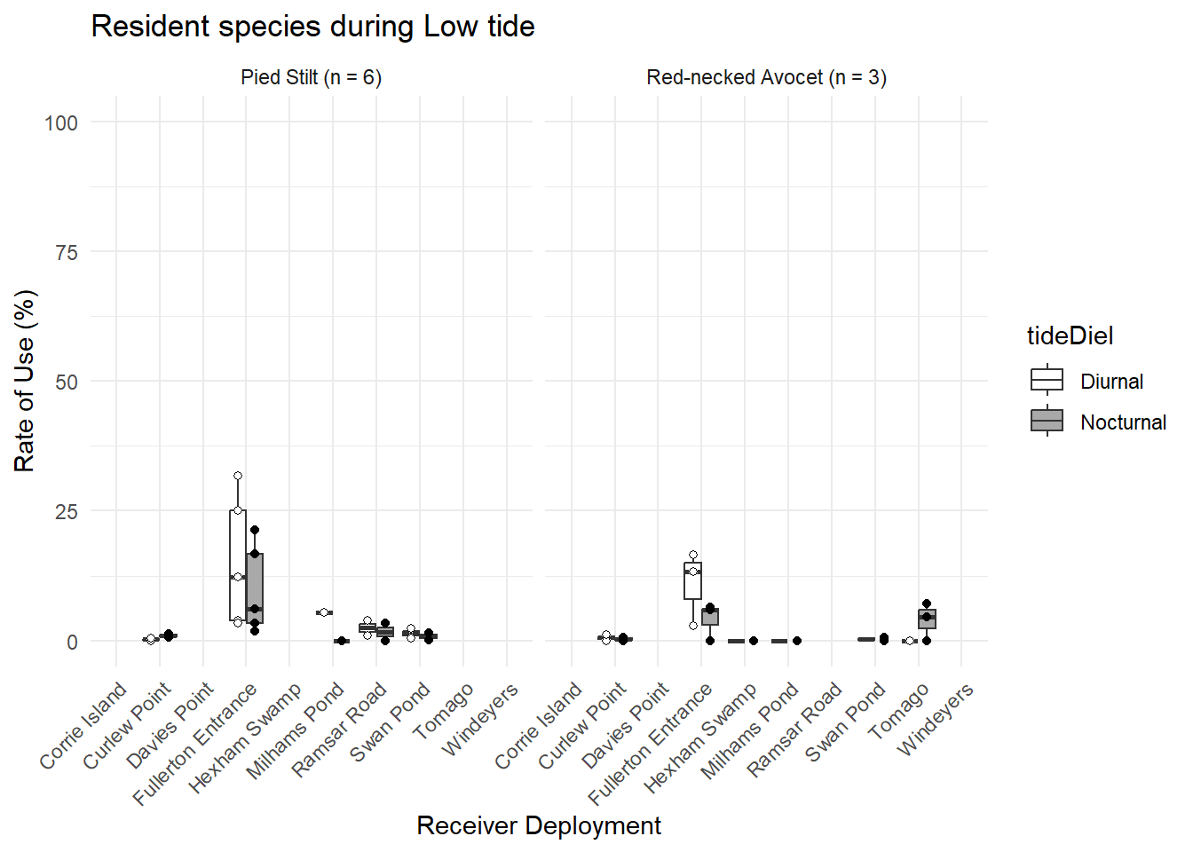
Low Tide Resident birds
| Statistics - Low Tide Resident Species | ||||||||||
|---|---|---|---|---|---|---|---|---|---|---|
| Species | Station | condition | n_individual | min | q1 | median | q3 | max | mean | sd |
| Pied Stilt | Corrie Island | Diurnal | 3 | Inf | NA | NA | NA | -Inf | NaN | NA |
| Pied Stilt | Corrie Island | Nocturnal | 3 | Inf | NA | NA | NA | -Inf | NaN | NA |
| Pied Stilt | Curlew Point | Diurnal | 4 | 0.0 | 0.1 | 0.2 | 0.3 | 0.4 | 0.2 | 0.3 |
| Pied Stilt | Curlew Point | Nocturnal | 4 | 0.7 | 0.8 | 1.0 | 1.1 | 1.3 | 1.0 | 0.4 |
| Pied Stilt | Davies Point | Diurnal | 3 | Inf | NA | NA | NA | -Inf | NaN | NA |
| Pied Stilt | Davies Point | Nocturnal | 3 | Inf | NA | NA | NA | -Inf | NaN | NA |
| Pied Stilt | Fullerton Entrance | Diurnal | 6 | 3.4 | 3.8 | 12.2 | 25.0 | 31.7 | 15.2 | 12.7 |
| Pied Stilt | Fullerton Entrance | Nocturnal | 6 | 1.8 | 3.3 | 6.2 | 16.7 | 21.3 | 9.8 | 8.7 |
| Pied Stilt | Hexham Swamp | Diurnal | 3 | Inf | NA | NA | NA | -Inf | NaN | NA |
| Pied Stilt | Hexham Swamp | Nocturnal | 3 | Inf | NA | NA | NA | -Inf | NaN | NA |
| Pied Stilt | Milhams Pond | Diurnal | 6 | 5.4 | 5.4 | 5.4 | 5.4 | 5.4 | 5.4 | NA |
| Pied Stilt | Milhams Pond | Nocturnal | 6 | 0.0 | 0.0 | 0.0 | 0.0 | 0.0 | 0.0 | NA |
| Pied Stilt | Ramsar Road | Diurnal | 6 | 0.9 | 1.7 | 2.4 | 3.2 | 3.9 | 2.4 | 2.2 |
| Pied Stilt | Ramsar Road | Nocturnal | 6 | 0.0 | 0.8 | 1.7 | 2.5 | 3.3 | 1.7 | 2.3 |
| Pied Stilt | Swan Pond | Diurnal | 6 | 0.5 | 0.9 | 1.4 | 1.8 | 2.3 | 1.4 | 1.3 |
| Pied Stilt | Swan Pond | Nocturnal | 6 | 0.2 | 0.5 | 0.8 | 1.1 | 1.4 | 0.8 | 0.9 |
| Pied Stilt | Tomago | Diurnal | 3 | Inf | NA | NA | NA | -Inf | NaN | NA |
| Pied Stilt | Tomago | Nocturnal | 3 | Inf | NA | NA | NA | -Inf | NaN | NA |
| Pied Stilt | Windeyers | Diurnal | 1 | Inf | NA | NA | NA | -Inf | NaN | NA |
| Pied Stilt | Windeyers | Nocturnal | 1 | Inf | NA | NA | NA | -Inf | NaN | NA |
| Red-necked Avocet | Corrie Island | Diurnal | 3 | Inf | NA | NA | NA | -Inf | NaN | NA |
| Red-necked Avocet | Corrie Island | Nocturnal | 3 | Inf | NA | NA | NA | -Inf | NaN | NA |
| Red-necked Avocet | Curlew Point | Diurnal | 3 | 0.0 | 0.3 | 0.6 | 0.8 | 1.1 | 0.6 | 0.8 |
| Red-necked Avocet | Curlew Point | Nocturnal | 3 | 0.0 | 0.2 | 0.3 | 0.5 | 0.6 | 0.3 | 0.5 |
| Red-necked Avocet | Davies Point | Diurnal | 3 | Inf | NA | NA | NA | -Inf | NaN | NA |
| Red-necked Avocet | Davies Point | Nocturnal | 3 | Inf | NA | NA | NA | -Inf | NaN | NA |
| Red-necked Avocet | Fullerton Entrance | Diurnal | 3 | 2.8 | 8.0 | 13.3 | 14.9 | 16.6 | 10.9 | 7.2 |
| Red-necked Avocet | Fullerton Entrance | Nocturnal | 3 | 0.0 | 2.9 | 5.8 | 6.2 | 6.5 | 4.1 | 3.6 |
| Red-necked Avocet | Hexham Swamp | Diurnal | 3 | Inf | NA | NA | NA | -Inf | NaN | NA |
| Red-necked Avocet | Hexham Swamp | Nocturnal | 3 | 0.0 | 0.0 | 0.0 | 0.0 | 0.0 | 0.0 | NA |
| Red-necked Avocet | Milhams Pond | Diurnal | 3 | Inf | NA | NA | NA | -Inf | NaN | NA |
| Red-necked Avocet | Milhams Pond | Nocturnal | 3 | 0.0 | 0.0 | 0.0 | 0.0 | 0.0 | 0.0 | NA |
| Red-necked Avocet | Ramsar Road | Diurnal | 3 | Inf | NA | NA | NA | -Inf | NaN | NA |
| Red-necked Avocet | Ramsar Road | Nocturnal | 3 | Inf | NA | NA | NA | -Inf | NaN | NA |
| Red-necked Avocet | Swan Pond | Diurnal | 3 | Inf | NA | NA | NA | -Inf | NaN | NA |
| Red-necked Avocet | Swan Pond | Nocturnal | 3 | 0.0 | 0.2 | 0.3 | 0.5 | 0.6 | 0.3 | 0.5 |
| Red-necked Avocet | Tomago | Diurnal | 3 | 0.0 | 0.0 | 0.0 | 0.0 | 0.0 | 0.0 | 0.0 |
| Red-necked Avocet | Tomago | Nocturnal | 3 | 0.0 | 2.3 | 4.5 | 5.8 | 7.1 | 3.9 | 3.6 |
MIGRATORY BIRDS
High Tide Migratory birds
| Statistics - High Tide Migratory Species | ||||||||||
|---|---|---|---|---|---|---|---|---|---|---|
| Species | Station | condition | n_individual | min | q1 | median | q3 | max | mean | sd |
| Bar-tailed Godwit | Corrie Island | Diurnal | 7 | Inf | NA | NA | NA | -Inf | NaN | NA |
| Bar-tailed Godwit | Corrie Island | Nocturnal | 7 | Inf | NA | NA | NA | -Inf | NaN | NA |
| Bar-tailed Godwit | Curlew Point | Diurnal | 8 | 1.2 | 36.8 | 59.8 | 81.5 | 100.0 | 56.4 | 36.4 |
| Bar-tailed Godwit | Curlew Point | Nocturnal | 8 | 0.4 | 9.8 | 11.3 | 67.3 | 100.0 | 36.4 | 44.2 |
| Bar-tailed Godwit | Davies Point | Diurnal | 7 | Inf | NA | NA | NA | -Inf | NaN | NA |
| Bar-tailed Godwit | Davies Point | Nocturnal | 7 | Inf | NA | NA | NA | -Inf | NaN | NA |
| Bar-tailed Godwit | Fullerton Entrance | Diurnal | 9 | 0.0 | 0.0 | 0.0 | 0.0 | 4.2 | 0.8 | 1.9 |
| Bar-tailed Godwit | Fullerton Entrance | Nocturnal | 9 | 0.0 | 0.0 | 0.0 | 0.0 | 0.0 | 0.0 | 0.0 |
| Bar-tailed Godwit | Hexham Swamp | Diurnal | 7 | Inf | NA | NA | NA | -Inf | NaN | NA |
| Bar-tailed Godwit | Hexham Swamp | Nocturnal | 7 | Inf | NA | NA | NA | -Inf | NaN | NA |
| Bar-tailed Godwit | Milhams Pond | Diurnal | 10 | Inf | NA | NA | NA | -Inf | NaN | NA |
| Bar-tailed Godwit | Milhams Pond | Nocturnal | 10 | 0.0 | 0.0 | 0.0 | 0.0 | 0.0 | 0.0 | NA |
| Bar-tailed Godwit | Ramsar Road | Diurnal | 9 | Inf | NA | NA | NA | -Inf | NaN | NA |
| Bar-tailed Godwit | Ramsar Road | Nocturnal | 9 | Inf | NA | NA | NA | -Inf | NaN | NA |
| Bar-tailed Godwit | Swan Pond | Diurnal | 10 | Inf | NA | NA | NA | -Inf | NaN | NA |
| Bar-tailed Godwit | Swan Pond | Nocturnal | 10 | Inf | NA | NA | NA | -Inf | NaN | NA |
| Bar-tailed Godwit | Tomago | Diurnal | 7 | 5.1 | 5.2 | 5.4 | 5.5 | 5.6 | 5.4 | 0.4 |
| Bar-tailed Godwit | Tomago | Nocturnal | 7 | 0.0 | 0.7 | 49.6 | 98.7 | 100.0 | 49.8 | 57.0 |
| Bar-tailed Godwit | Windeyers | Diurnal | 4 | Inf | NA | NA | NA | -Inf | NaN | NA |
| Bar-tailed Godwit | Windeyers | Nocturnal | 4 | Inf | NA | NA | NA | -Inf | NaN | NA |
| Curlew Sandpiper | Corrie Island | Diurnal | 5 | Inf | NA | NA | NA | -Inf | NaN | NA |
| Curlew Sandpiper | Corrie Island | Nocturnal | 5 | Inf | NA | NA | NA | -Inf | NaN | NA |
| Curlew Sandpiper | Curlew Point | Diurnal | 5 | 12.2 | 22.7 | 39.8 | 42.8 | 43.0 | 32.1 | 13.9 |
| Curlew Sandpiper | Curlew Point | Nocturnal | 5 | 2.0 | 9.7 | 10.1 | 11.3 | 15.7 | 9.8 | 5.0 |
| Curlew Sandpiper | Davies Point | Diurnal | 5 | Inf | NA | NA | NA | -Inf | NaN | NA |
| Curlew Sandpiper | Davies Point | Nocturnal | 5 | Inf | NA | NA | NA | -Inf | NaN | NA |
| Curlew Sandpiper | Fullerton Entrance | Diurnal | 5 | 0.0 | 0.0 | 0.0 | 0.0 | 0.0 | 0.0 | 0.0 |
| Curlew Sandpiper | Fullerton Entrance | Nocturnal | 5 | 0.0 | 0.0 | 0.0 | 0.0 | 0.0 | 0.0 | 0.0 |
| Curlew Sandpiper | Hexham Swamp | Diurnal | 5 | Inf | NA | NA | NA | -Inf | NaN | NA |
| Curlew Sandpiper | Hexham Swamp | Nocturnal | 5 | Inf | NA | NA | NA | -Inf | NaN | NA |
| Curlew Sandpiper | Milhams Pond | Diurnal | 5 | 0.0 | 0.0 | 0.0 | 0.0 | 0.0 | 0.0 | NA |
| Curlew Sandpiper | Milhams Pond | Nocturnal | 5 | 0.0 | 0.0 | 0.0 | 0.0 | 0.0 | 0.0 | NA |
| Curlew Sandpiper | Ramsar Road | Diurnal | 5 | 0.0 | 0.0 | 0.0 | 0.0 | 0.0 | 0.0 | 0.0 |
| Curlew Sandpiper | Ramsar Road | Nocturnal | 5 | 0.0 | 0.0 | 0.1 | 0.2 | 0.2 | 0.1 | 0.1 |
| Curlew Sandpiper | Swan Pond | Diurnal | 5 | 0.0 | 0.0 | 0.1 | 0.1 | 0.1 | 0.1 | 0.1 |
| Curlew Sandpiper | Swan Pond | Nocturnal | 5 | 0.0 | 0.0 | 0.2 | 0.2 | 0.2 | 0.1 | 0.1 |
| Curlew Sandpiper | Tomago | Diurnal | 5 | 0.0 | 0.0 | 0.0 | 0.0 | 0.1 | 0.0 | 0.1 |
| Curlew Sandpiper | Tomago | Nocturnal | 5 | 0.0 | 0.0 | 0.0 | 0.2 | 0.2 | 0.1 | 0.1 |
| Curlew Sandpiper | Windeyers | Diurnal | 5 | Inf | NA | NA | NA | -Inf | NaN | NA |
| Curlew Sandpiper | Windeyers | Nocturnal | 5 | Inf | NA | NA | NA | -Inf | NaN | NA |
| Eurasian Whimbrel | Corrie Island | Diurnal | 2 | Inf | NA | NA | NA | -Inf | NaN | NA |
| Eurasian Whimbrel | Corrie Island | Nocturnal | 2 | Inf | NA | NA | NA | -Inf | NaN | NA |
| Eurasian Whimbrel | Curlew Point | Diurnal | 2 | 0.0 | 0.5 | 0.9 | 1.4 | 1.9 | 0.9 | 1.3 |
| Eurasian Whimbrel | Curlew Point | Nocturnal | 2 | 0.0 | 1.1 | 2.2 | 3.3 | 4.4 | 2.2 | 3.1 |
| Eurasian Whimbrel | Davies Point | Diurnal | 2 | Inf | NA | NA | NA | -Inf | NaN | NA |
| Eurasian Whimbrel | Davies Point | Nocturnal | 2 | Inf | NA | NA | NA | -Inf | NaN | NA |
| Eurasian Whimbrel | Fullerton Entrance | Diurnal | 2 | 2.9 | 3.3 | 3.6 | 4.0 | 4.4 | 3.6 | 1.0 |
| Eurasian Whimbrel | Fullerton Entrance | Nocturnal | 2 | 0.0 | 0.0 | 0.0 | 0.0 | 0.0 | 0.0 | 0.0 |
| Eurasian Whimbrel | Hexham Swamp | Diurnal | 2 | Inf | NA | NA | NA | -Inf | NaN | NA |
| Eurasian Whimbrel | Hexham Swamp | Nocturnal | 2 | Inf | NA | NA | NA | -Inf | NaN | NA |
| Eurasian Whimbrel | Milhams Pond | Diurnal | 2 | Inf | NA | NA | NA | -Inf | NaN | NA |
| Eurasian Whimbrel | Milhams Pond | Nocturnal | 2 | Inf | NA | NA | NA | -Inf | NaN | NA |
| Eurasian Whimbrel | Ramsar Road | Diurnal | 2 | Inf | NA | NA | NA | -Inf | NaN | NA |
| Eurasian Whimbrel | Ramsar Road | Nocturnal | 2 | Inf | NA | NA | NA | -Inf | NaN | NA |
| Eurasian Whimbrel | Swan Pond | Diurnal | 2 | Inf | NA | NA | NA | -Inf | NaN | NA |
| Eurasian Whimbrel | Swan Pond | Nocturnal | 2 | Inf | NA | NA | NA | -Inf | NaN | NA |
| Eurasian Whimbrel | Tomago | Diurnal | 2 | Inf | NA | NA | NA | -Inf | NaN | NA |
| Eurasian Whimbrel | Tomago | Nocturnal | 2 | 0.8 | 0.8 | 0.8 | 0.8 | 0.8 | 0.8 | NA |
| Eurasian Whimbrel | Windeyers | Diurnal | 2 | Inf | NA | NA | NA | -Inf | NaN | NA |
| Eurasian Whimbrel | Windeyers | Nocturnal | 2 | Inf | NA | NA | NA | -Inf | NaN | NA |
| Far Eastern Curlew | Corrie Island | Diurnal | 1 | Inf | NA | NA | NA | -Inf | NaN | NA |
| Far Eastern Curlew | Corrie Island | Nocturnal | 1 | Inf | NA | NA | NA | -Inf | NaN | NA |
| Far Eastern Curlew | Curlew Point | Diurnal | 1 | 1.2 | 1.2 | 1.2 | 1.2 | 1.2 | 1.2 | NA |
| Far Eastern Curlew | Curlew Point | Nocturnal | 1 | Inf | NA | NA | NA | -Inf | NaN | NA |
| Far Eastern Curlew | Davies Point | Diurnal | 1 | Inf | NA | NA | NA | -Inf | NaN | NA |
| Far Eastern Curlew | Davies Point | Nocturnal | 1 | Inf | NA | NA | NA | -Inf | NaN | NA |
| Far Eastern Curlew | Fullerton Entrance | Diurnal | 2 | 0.0 | 0.0 | 0.0 | 0.0 | 0.0 | 0.0 | NA |
| Far Eastern Curlew | Fullerton Entrance | Nocturnal | 2 | 0.0 | 0.0 | 0.0 | 0.0 | 0.0 | 0.0 | 0.0 |
| Far Eastern Curlew | Hexham Swamp | Diurnal | 1 | Inf | NA | NA | NA | -Inf | NaN | NA |
| Far Eastern Curlew | Hexham Swamp | Nocturnal | 1 | Inf | NA | NA | NA | -Inf | NaN | NA |
| Far Eastern Curlew | Milhams Pond | Diurnal | 2 | 18.0 | 18.0 | 18.0 | 18.0 | 18.0 | 18.0 | NA |
| Far Eastern Curlew | Milhams Pond | Nocturnal | 2 | 8.5 | 8.5 | 8.5 | 8.5 | 8.5 | 8.5 | NA |
| Far Eastern Curlew | Ramsar Road | Diurnal | 2 | Inf | NA | NA | NA | -Inf | NaN | NA |
| Far Eastern Curlew | Ramsar Road | Nocturnal | 2 | Inf | NA | NA | NA | -Inf | NaN | NA |
| Far Eastern Curlew | Swan Pond | Diurnal | 2 | Inf | NA | NA | NA | -Inf | NaN | NA |
| Far Eastern Curlew | Swan Pond | Nocturnal | 2 | Inf | NA | NA | NA | -Inf | NaN | NA |
| Far Eastern Curlew | Tomago | Diurnal | 1 | Inf | NA | NA | NA | -Inf | NaN | NA |
| Far Eastern Curlew | Tomago | Nocturnal | 1 | 1.4 | 1.4 | 1.4 | 1.4 | 1.4 | 1.4 | NA |
| Far Eastern Curlew | Windeyers | Diurnal | 1 | Inf | NA | NA | NA | -Inf | NaN | NA |
| Far Eastern Curlew | Windeyers | Nocturnal | 1 | Inf | NA | NA | NA | -Inf | NaN | NA |
| Pacific Golden-Plover | Corrie Island | Diurnal | 14 | Inf | NA | NA | NA | -Inf | NaN | NA |
| Pacific Golden-Plover | Corrie Island | Nocturnal | 14 | Inf | NA | NA | NA | -Inf | NaN | NA |
| Pacific Golden-Plover | Curlew Point | Diurnal | 14 | 0.0 | 5.0 | 13.3 | 60.2 | 100.0 | 31.5 | 34.8 |
| Pacific Golden-Plover | Curlew Point | Nocturnal | 14 | 0.0 | 0.0 | 2.6 | 11.6 | 22.3 | 6.2 | 7.4 |
| Pacific Golden-Plover | Davies Point | Diurnal | 14 | Inf | NA | NA | NA | -Inf | NaN | NA |
| Pacific Golden-Plover | Davies Point | Nocturnal | 14 | Inf | NA | NA | NA | -Inf | NaN | NA |
| Pacific Golden-Plover | Fullerton Entrance | Diurnal | 14 | 0.0 | 0.0 | 0.0 | 0.0 | 0.4 | 0.1 | 0.1 |
| Pacific Golden-Plover | Fullerton Entrance | Nocturnal | 14 | 0.0 | 0.0 | 0.0 | 0.3 | 0.9 | 0.2 | 0.4 |
| Pacific Golden-Plover | Hexham Swamp | Diurnal | 14 | 0.0 | 0.0 | 1.9 | 5.8 | 11.0 | 3.5 | 4.2 |
| Pacific Golden-Plover | Hexham Swamp | Nocturnal | 14 | 0.0 | 0.0 | 0.9 | 1.4 | 3.1 | 1.0 | 1.1 |
| Pacific Golden-Plover | Milhams Pond | Diurnal | 14 | 0.0 | 0.0 | 0.0 | 42.8 | 85.6 | 28.5 | 49.4 |
| Pacific Golden-Plover | Milhams Pond | Nocturnal | 14 | 0.0 | 0.0 | 0.0 | 11.7 | 46.7 | 11.7 | 23.4 |
| Pacific Golden-Plover | Ramsar Road | Diurnal | 14 | 0.0 | 0.0 | 0.0 | 0.0 | 0.6 | 0.1 | 0.3 |
| Pacific Golden-Plover | Ramsar Road | Nocturnal | 14 | 0.0 | 0.0 | 0.0 | 0.0 | 1.3 | 0.2 | 0.5 |
| Pacific Golden-Plover | Swan Pond | Diurnal | 14 | 0.0 | 0.0 | 0.0 | 0.0 | 0.2 | 0.0 | 0.1 |
| Pacific Golden-Plover | Swan Pond | Nocturnal | 14 | 0.0 | 0.0 | 0.0 | 0.0 | 0.6 | 0.1 | 0.2 |
| Pacific Golden-Plover | Tomago | Diurnal | 14 | Inf | NA | NA | NA | -Inf | NaN | NA |
| Pacific Golden-Plover | Tomago | Nocturnal | 14 | Inf | NA | NA | NA | -Inf | NaN | NA |
| Pacific Golden-Plover | Windeyers | Diurnal | 12 | 0.0 | 0.0 | 0.0 | 0.0 | 0.0 | 0.0 | 0.0 |
| Pacific Golden-Plover | Windeyers | Nocturnal | 12 | 0.0 | 0.0 | 0.0 | 0.3 | 1.1 | 0.3 | 0.6 |
Low Tide Migratory birds
| Statistics - Low Tide Migratory Species | ||||||||||
|---|---|---|---|---|---|---|---|---|---|---|
| Species | Station | condition | n_individual | min | q1 | median | q3 | max | mean | sd |
| Bar-tailed Godwit | Corrie Island | Diurnal | 7 | Inf | NA | NA | NA | -Inf | NaN | NA |
| Bar-tailed Godwit | Corrie Island | Nocturnal | 7 | Inf | NA | NA | NA | -Inf | NaN | NA |
| Bar-tailed Godwit | Curlew Point | Diurnal | 8 | 0.0 | 0.8 | 3.8 | 6.1 | 83.3 | 16.3 | 33.0 |
| Bar-tailed Godwit | Curlew Point | Nocturnal | 8 | 0.0 | 0.6 | 1.3 | 3.4 | 25.0 | 6.0 | 10.7 |
| Bar-tailed Godwit | Davies Point | Diurnal | 7 | Inf | NA | NA | NA | -Inf | NaN | NA |
| Bar-tailed Godwit | Davies Point | Nocturnal | 7 | Inf | NA | NA | NA | -Inf | NaN | NA |
| Bar-tailed Godwit | Fullerton Entrance | Diurnal | 9 | 0.0 | 0.0 | 0.0 | 0.0 | 0.0 | 0.0 | 0.0 |
| Bar-tailed Godwit | Fullerton Entrance | Nocturnal | 9 | 0.0 | 0.0 | 0.4 | 0.9 | 1.3 | 0.5 | 0.6 |
| Bar-tailed Godwit | Hexham Swamp | Diurnal | 7 | Inf | NA | NA | NA | -Inf | NaN | NA |
| Bar-tailed Godwit | Hexham Swamp | Nocturnal | 7 | Inf | NA | NA | NA | -Inf | NaN | NA |
| Bar-tailed Godwit | Milhams Pond | Diurnal | 10 | 0.0 | 0.0 | 0.0 | 0.0 | 0.0 | 0.0 | 0.0 |
| Bar-tailed Godwit | Milhams Pond | Nocturnal | 10 | 0.0 | 0.0 | 0.0 | 0.0 | 0.0 | 0.0 | NA |
| Bar-tailed Godwit | Ramsar Road | Diurnal | 9 | Inf | NA | NA | NA | -Inf | NaN | NA |
| Bar-tailed Godwit | Ramsar Road | Nocturnal | 9 | Inf | NA | NA | NA | -Inf | NaN | NA |
| Bar-tailed Godwit | Swan Pond | Diurnal | 10 | Inf | NA | NA | NA | -Inf | NaN | NA |
| Bar-tailed Godwit | Swan Pond | Nocturnal | 10 | Inf | NA | NA | NA | -Inf | NaN | NA |
| Bar-tailed Godwit | Tomago | Diurnal | 7 | 0.0 | 0.0 | 0.0 | 0.0 | 0.0 | 0.0 | NA |
| Bar-tailed Godwit | Tomago | Nocturnal | 7 | 0.1 | 6.3 | 12.5 | 19.3 | 27.1 | 13.0 | 11.6 |
| Bar-tailed Godwit | Windeyers | Diurnal | 4 | Inf | NA | NA | NA | -Inf | NaN | NA |
| Bar-tailed Godwit | Windeyers | Nocturnal | 4 | Inf | NA | NA | NA | -Inf | NaN | NA |
| Curlew Sandpiper | Corrie Island | Diurnal | 5 | Inf | NA | NA | NA | -Inf | NaN | NA |
| Curlew Sandpiper | Corrie Island | Nocturnal | 5 | Inf | NA | NA | NA | -Inf | NaN | NA |
| Curlew Sandpiper | Curlew Point | Diurnal | 5 | 10.4 | 24.3 | 30.6 | 30.8 | 34.0 | 26.0 | 9.4 |
| Curlew Sandpiper | Curlew Point | Nocturnal | 5 | 3.2 | 9.2 | 11.0 | 11.6 | 14.3 | 9.8 | 4.2 |
| Curlew Sandpiper | Davies Point | Diurnal | 5 | Inf | NA | NA | NA | -Inf | NaN | NA |
| Curlew Sandpiper | Davies Point | Nocturnal | 5 | Inf | NA | NA | NA | -Inf | NaN | NA |
| Curlew Sandpiper | Fullerton Entrance | Diurnal | 5 | 0.0 | 0.0 | 0.0 | 0.0 | 0.0 | 0.0 | 0.0 |
| Curlew Sandpiper | Fullerton Entrance | Nocturnal | 5 | 0.0 | 0.2 | 0.2 | 0.2 | 0.3 | 0.2 | 0.1 |
| Curlew Sandpiper | Hexham Swamp | Diurnal | 5 | Inf | NA | NA | NA | -Inf | NaN | NA |
| Curlew Sandpiper | Hexham Swamp | Nocturnal | 5 | Inf | NA | NA | NA | -Inf | NaN | NA |
| Curlew Sandpiper | Milhams Pond | Diurnal | 5 | 0.0 | 0.0 | 0.0 | 0.0 | 0.0 | 0.0 | NA |
| Curlew Sandpiper | Milhams Pond | Nocturnal | 5 | 0.0 | 0.0 | 0.0 | 0.0 | 0.0 | 0.0 | 0.0 |
| Curlew Sandpiper | Ramsar Road | Diurnal | 5 | 0.0 | 0.0 | 0.0 | 0.0 | 0.0 | 0.0 | 0.0 |
| Curlew Sandpiper | Ramsar Road | Nocturnal | 5 | 0.0 | 0.1 | 0.2 | 0.2 | 0.2 | 0.1 | 0.1 |
| Curlew Sandpiper | Swan Pond | Diurnal | 5 | 0.0 | 0.0 | 0.0 | 0.0 | 0.1 | 0.0 | 0.1 |
| Curlew Sandpiper | Swan Pond | Nocturnal | 5 | 0.0 | 0.2 | 0.2 | 0.3 | 0.3 | 0.2 | 0.1 |
| Curlew Sandpiper | Tomago | Diurnal | 5 | 0.0 | 0.0 | 0.0 | 0.0 | 0.0 | 0.0 | 0.0 |
| Curlew Sandpiper | Tomago | Nocturnal | 5 | 0.0 | 0.0 | 0.2 | 0.2 | 0.3 | 0.1 | 0.1 |
| Curlew Sandpiper | Windeyers | Diurnal | 5 | Inf | NA | NA | NA | -Inf | NaN | NA |
| Curlew Sandpiper | Windeyers | Nocturnal | 5 | Inf | NA | NA | NA | -Inf | NaN | NA |
| Eurasian Whimbrel | Corrie Island | Diurnal | 2 | Inf | NA | NA | NA | -Inf | NaN | NA |
| Eurasian Whimbrel | Corrie Island | Nocturnal | 2 | Inf | NA | NA | NA | -Inf | NaN | NA |
| Eurasian Whimbrel | Curlew Point | Diurnal | 2 | 1.4 | 1.4 | 1.4 | 1.4 | 1.4 | 1.4 | NA |
| Eurasian Whimbrel | Curlew Point | Nocturnal | 2 | 1.1 | 2.7 | 4.2 | 5.7 | 7.2 | 4.2 | 4.3 |
| Eurasian Whimbrel | Davies Point | Diurnal | 2 | Inf | NA | NA | NA | -Inf | NaN | NA |
| Eurasian Whimbrel | Davies Point | Nocturnal | 2 | Inf | NA | NA | NA | -Inf | NaN | NA |
| Eurasian Whimbrel | Fullerton Entrance | Diurnal | 2 | 0.0 | 0.1 | 0.2 | 0.3 | 0.4 | 0.2 | 0.3 |
| Eurasian Whimbrel | Fullerton Entrance | Nocturnal | 2 | 0.0 | 0.0 | 0.0 | 0.0 | 0.0 | 0.0 | 0.0 |
| Eurasian Whimbrel | Hexham Swamp | Diurnal | 2 | Inf | NA | NA | NA | -Inf | NaN | NA |
| Eurasian Whimbrel | Hexham Swamp | Nocturnal | 2 | Inf | NA | NA | NA | -Inf | NaN | NA |
| Eurasian Whimbrel | Milhams Pond | Diurnal | 2 | Inf | NA | NA | NA | -Inf | NaN | NA |
| Eurasian Whimbrel | Milhams Pond | Nocturnal | 2 | Inf | NA | NA | NA | -Inf | NaN | NA |
| Eurasian Whimbrel | Ramsar Road | Diurnal | 2 | Inf | NA | NA | NA | -Inf | NaN | NA |
| Eurasian Whimbrel | Ramsar Road | Nocturnal | 2 | Inf | NA | NA | NA | -Inf | NaN | NA |
| Eurasian Whimbrel | Swan Pond | Diurnal | 2 | Inf | NA | NA | NA | -Inf | NaN | NA |
| Eurasian Whimbrel | Swan Pond | Nocturnal | 2 | Inf | NA | NA | NA | -Inf | NaN | NA |
| Eurasian Whimbrel | Tomago | Diurnal | 2 | 0.0 | 0.0 | 0.0 | 0.0 | 0.0 | 0.0 | NA |
| Eurasian Whimbrel | Tomago | Nocturnal | 2 | 0.6 | 0.6 | 0.6 | 0.6 | 0.6 | 0.6 | NA |
| Eurasian Whimbrel | Windeyers | Diurnal | 2 | Inf | NA | NA | NA | -Inf | NaN | NA |
| Eurasian Whimbrel | Windeyers | Nocturnal | 2 | Inf | NA | NA | NA | -Inf | NaN | NA |
| Far Eastern Curlew | Corrie Island | Diurnal | 1 | Inf | NA | NA | NA | -Inf | NaN | NA |
| Far Eastern Curlew | Corrie Island | Nocturnal | 1 | Inf | NA | NA | NA | -Inf | NaN | NA |
| Far Eastern Curlew | Curlew Point | Diurnal | 1 | Inf | NA | NA | NA | -Inf | NaN | NA |
| Far Eastern Curlew | Curlew Point | Nocturnal | 1 | Inf | NA | NA | NA | -Inf | NaN | NA |
| Far Eastern Curlew | Davies Point | Diurnal | 1 | Inf | NA | NA | NA | -Inf | NaN | NA |
| Far Eastern Curlew | Davies Point | Nocturnal | 1 | Inf | NA | NA | NA | -Inf | NaN | NA |
| Far Eastern Curlew | Fullerton Entrance | Diurnal | 2 | 0.0 | 0.0 | 0.0 | 0.0 | 0.0 | 0.0 | NA |
| Far Eastern Curlew | Fullerton Entrance | Nocturnal | 2 | 0.0 | 0.0 | 0.0 | 0.0 | 0.0 | 0.0 | 0.0 |
| Far Eastern Curlew | Hexham Swamp | Diurnal | 1 | Inf | NA | NA | NA | -Inf | NaN | NA |
| Far Eastern Curlew | Hexham Swamp | Nocturnal | 1 | Inf | NA | NA | NA | -Inf | NaN | NA |
| Far Eastern Curlew | Milhams Pond | Diurnal | 2 | 19.6 | 19.6 | 19.6 | 19.6 | 19.6 | 19.6 | NA |
| Far Eastern Curlew | Milhams Pond | Nocturnal | 2 | 44.7 | 44.7 | 44.7 | 44.7 | 44.7 | 44.7 | NA |
| Far Eastern Curlew | Ramsar Road | Diurnal | 2 | Inf | NA | NA | NA | -Inf | NaN | NA |
| Far Eastern Curlew | Ramsar Road | Nocturnal | 2 | Inf | NA | NA | NA | -Inf | NaN | NA |
| Far Eastern Curlew | Swan Pond | Diurnal | 2 | Inf | NA | NA | NA | -Inf | NaN | NA |
| Far Eastern Curlew | Swan Pond | Nocturnal | 2 | Inf | NA | NA | NA | -Inf | NaN | NA |
| Far Eastern Curlew | Tomago | Diurnal | 1 | 0.0 | 0.0 | 0.0 | 0.0 | 0.0 | 0.0 | NA |
| Far Eastern Curlew | Tomago | Nocturnal | 1 | 1.5 | 1.5 | 1.5 | 1.5 | 1.5 | 1.5 | NA |
| Far Eastern Curlew | Windeyers | Diurnal | 1 | Inf | NA | NA | NA | -Inf | NaN | NA |
| Far Eastern Curlew | Windeyers | Nocturnal | 1 | Inf | NA | NA | NA | -Inf | NaN | NA |
| Pacific Golden-Plover | Corrie Island | Diurnal | 14 | Inf | NA | NA | NA | -Inf | NaN | NA |
| Pacific Golden-Plover | Corrie Island | Nocturnal | 14 | Inf | NA | NA | NA | -Inf | NaN | NA |
| Pacific Golden-Plover | Curlew Point | Diurnal | 14 | 3.6 | 9.9 | 13.2 | 53.9 | 100.0 | 31.9 | 33.4 |
| Pacific Golden-Plover | Curlew Point | Nocturnal | 14 | 0.0 | 2.0 | 4.2 | 19.2 | 38.8 | 10.0 | 12.2 |
| Pacific Golden-Plover | Davies Point | Diurnal | 14 | Inf | NA | NA | NA | -Inf | NaN | NA |
| Pacific Golden-Plover | Davies Point | Nocturnal | 14 | Inf | NA | NA | NA | -Inf | NaN | NA |
| Pacific Golden-Plover | Fullerton Entrance | Diurnal | 14 | 0.0 | 0.0 | 0.0 | 0.1 | 0.6 | 0.1 | 0.2 |
| Pacific Golden-Plover | Fullerton Entrance | Nocturnal | 14 | 0.0 | 0.0 | 0.0 | 0.2 | 1.0 | 0.2 | 0.4 |
| Pacific Golden-Plover | Hexham Swamp | Diurnal | 14 | 0.0 | 2.7 | 4.3 | 7.7 | 11.6 | 5.2 | 4.3 |
| Pacific Golden-Plover | Hexham Swamp | Nocturnal | 14 | 0.0 | 0.1 | 0.9 | 1.1 | 1.9 | 0.7 | 0.7 |
| Pacific Golden-Plover | Milhams Pond | Diurnal | 14 | 0.0 | 0.0 | 0.0 | 0.0 | 81.4 | 16.3 | 36.4 |
| Pacific Golden-Plover | Milhams Pond | Nocturnal | 14 | 0.0 | 0.0 | 1.2 | 15.7 | 55.9 | 14.5 | 27.6 |
| Pacific Golden-Plover | Ramsar Road | Diurnal | 14 | 0.0 | 0.0 | 0.0 | 0.0 | 1.3 | 0.2 | 0.5 |
| Pacific Golden-Plover | Ramsar Road | Nocturnal | 14 | 0.0 | 0.0 | 0.0 | 0.0 | 2.7 | 0.3 | 0.9 |
| Pacific Golden-Plover | Swan Pond | Diurnal | 14 | 0.0 | 0.0 | 0.0 | 0.0 | 0.0 | 0.0 | 0.0 |
| Pacific Golden-Plover | Swan Pond | Nocturnal | 14 | 0.0 | 0.0 | 0.0 | 0.0 | 0.0 | 0.0 | 0.0 |
| Pacific Golden-Plover | Tomago | Diurnal | 14 | 0.0 | 0.0 | 0.0 | 0.0 | 0.0 | 0.0 | NA |
| Pacific Golden-Plover | Tomago | Nocturnal | 14 | Inf | NA | NA | NA | -Inf | NaN | NA |
| Pacific Golden-Plover | Windeyers | Diurnal | 12 | 0.0 | 0.0 | 0.0 | 0.0 | 0.0 | 0.0 | 0.0 |
| Pacific Golden-Plover | Windeyers | Nocturnal | 12 | 0.0 | 0.0 | 0.0 | 0.1 | 0.5 | 0.1 | 0.3 |
Hourly usage
USED vs AVAILABLE
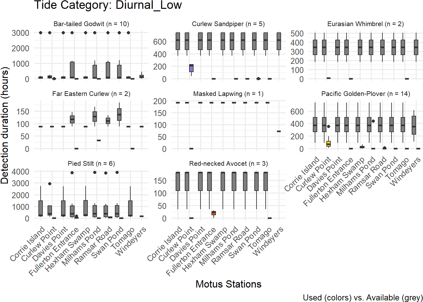
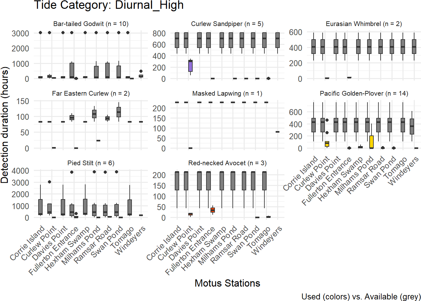
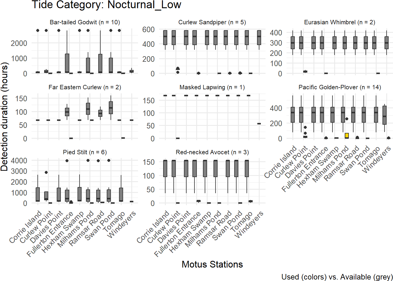
Legend: Shorebird movement and spatial ecology vary across species and within the local MOTUS array in NSW. Each tab displays one tide category from the pairs “high/low” and “nocturnal/diurnal,” showing used time in hours (colored boxes) for each species at different Motus stations. The grey boxes represent the total available time for the corresponding tide category and Motus station, across individuals. Note that available time might be relatively similar across stations as it is based on the general Newcastle tide table and is not station-specific.
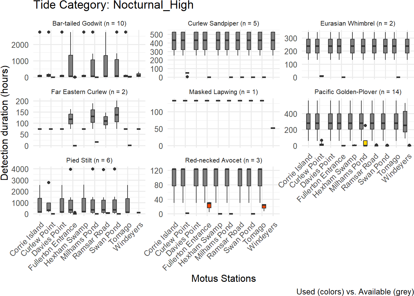
USED
Since the size sample at the current date is too low, it might be hard to read in details how much each bird or species spent time (hours) at each Motus station. So here below is displayed the used only for each stations.
# Plot function used ONLY
plot_used <- function(tide_cat) {
  data_subset <- used_bird_recv_time %>% filter(tideCategory == tide_cat)

  ggplot(data_subset,
         aes(x = recvDeployName, y = duration_h, fill = speciesEN)) +

    geom_boxplot(position = position_dodge2(width = 0.9, preserve = "single")) +
    scale_fill_manual(values = species_colors, name = "Species") +

    facet_wrap(~ speciesEN, scales = "free_y",
               labeller = labeller(speciesEN = label_vec)) +

    theme_minimal(base_size = 12) +
    theme(strip.text = element_text(face = "bold", size = 10),
          axis.text.x = element_text(angle = 45, hjust = 1),
          legend.position = "none",
          plot.margin = margin(0, 0, 0, 0, "in"))  +

    coord_cartesian(ylim = c(0, NA), expand = FALSE) +
    labs(x = "Motus stations",
         y = "Detection duration (hours)",
         title = paste("Tide Category:", tide_cat),
         fill = "Species")
  }

# Get unique tideCategory levels
tide_categories <- combined_data %>%
  filter(!is.na(tideCategory)) %>%
  pull(tideCategory) %>%
  unique()

# Generate a list of plots for all tide categories
plots_list_used <- purrr::map(tide_categories, plot_used)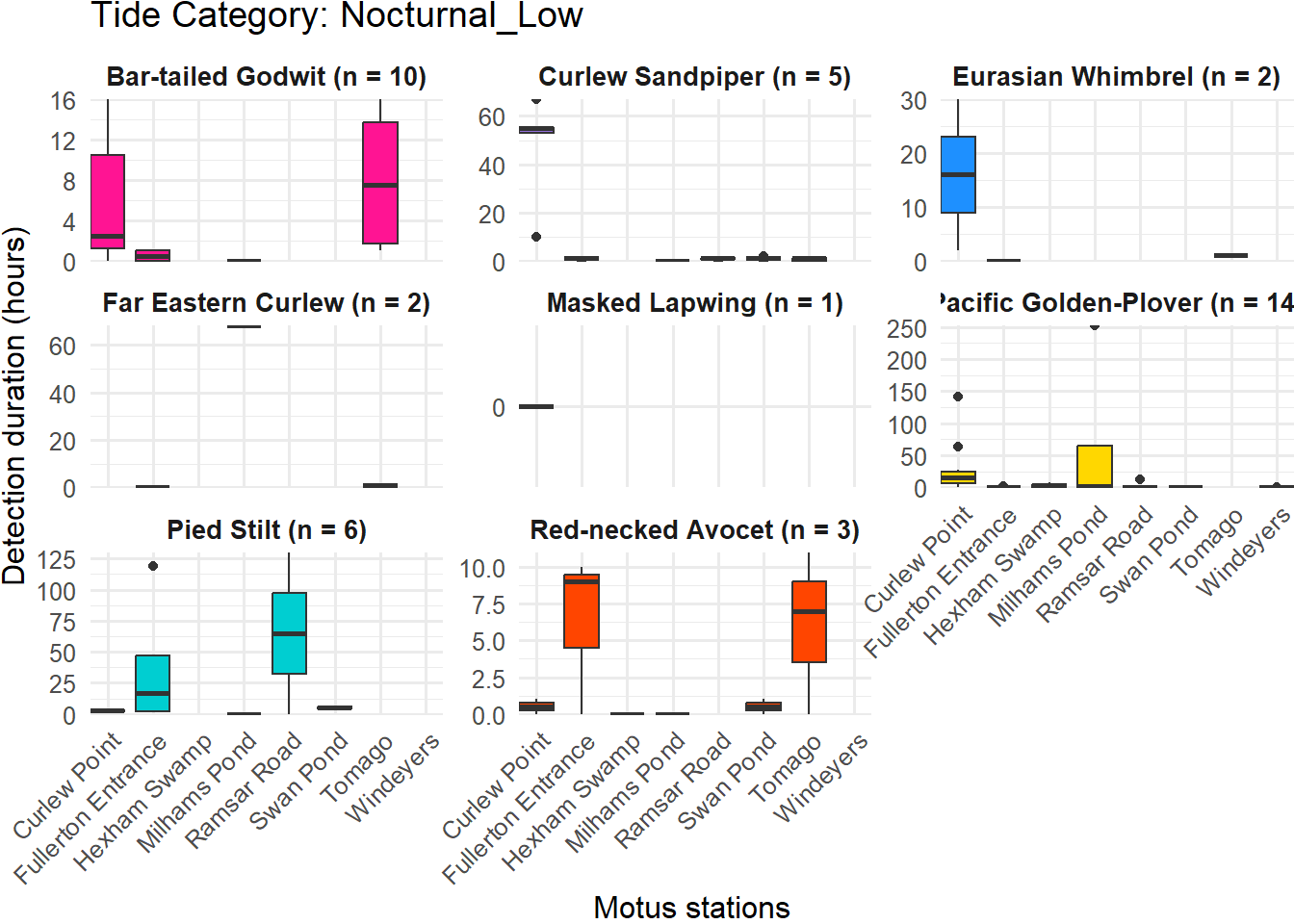
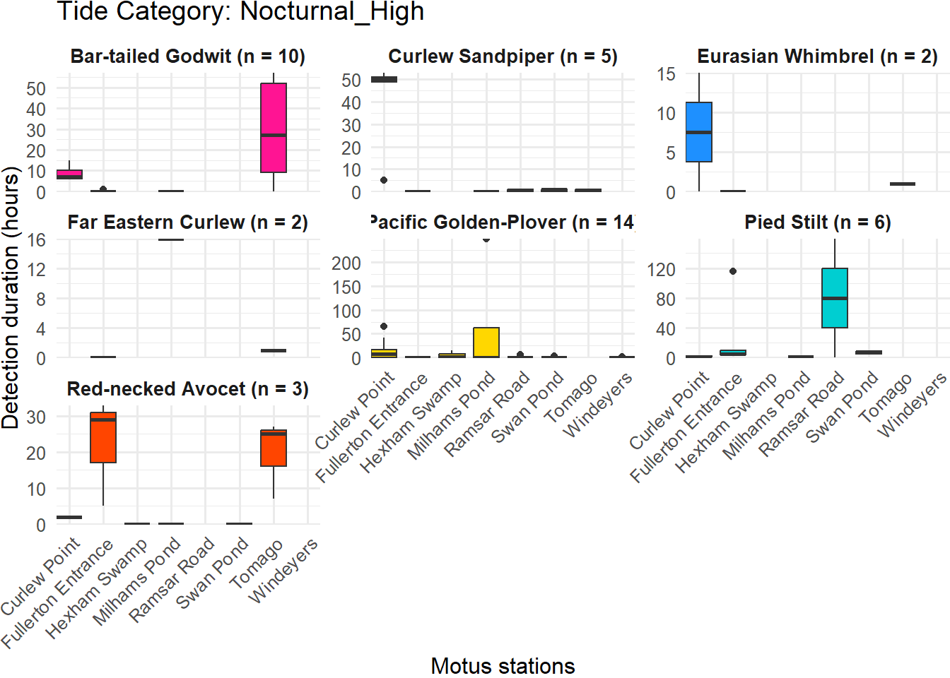
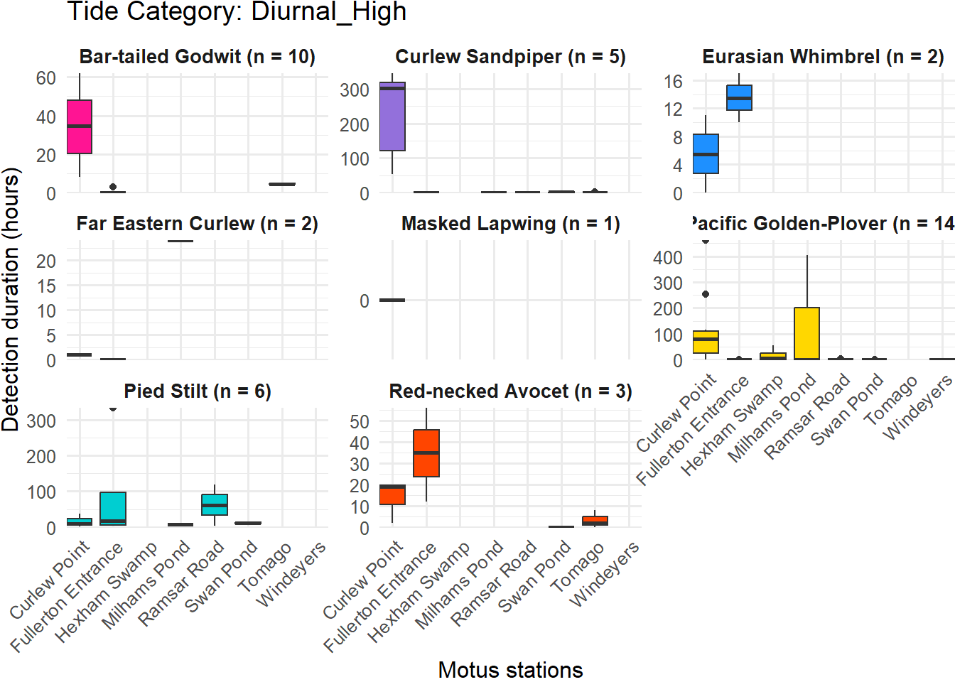
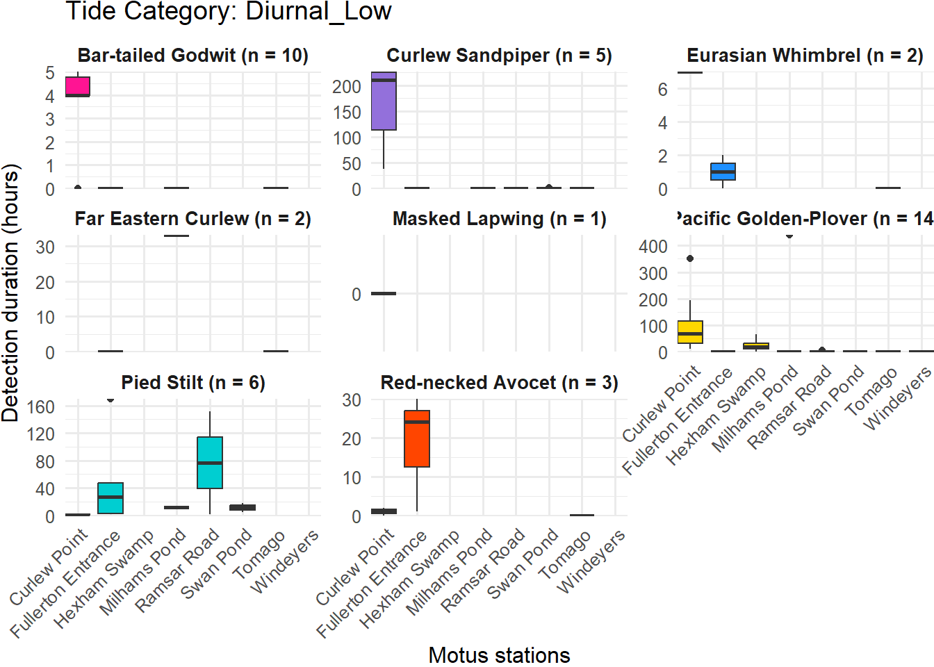
Legend: Shorebird movement and spatial ecology vary across species and within the local Motus array in NSW. Each tab displays one tide category from the pairs “high/low” and “nocturnal/diurnal,” showing how many hours each species have been recorded at different Motus stations.
Detection conditions
Visualise here the difference between the total number of hours recorded across the four tidal conditions for each species and for the whole population of tagged shorebirds, “Total used”. And see the difference with the “Usage rate”, which measures bird detections by the Motus array as a proportion of the total available detection time.
POPULATION
TOTAL SURVEY EFFORT (%) - TOTAL AVAILABLE -
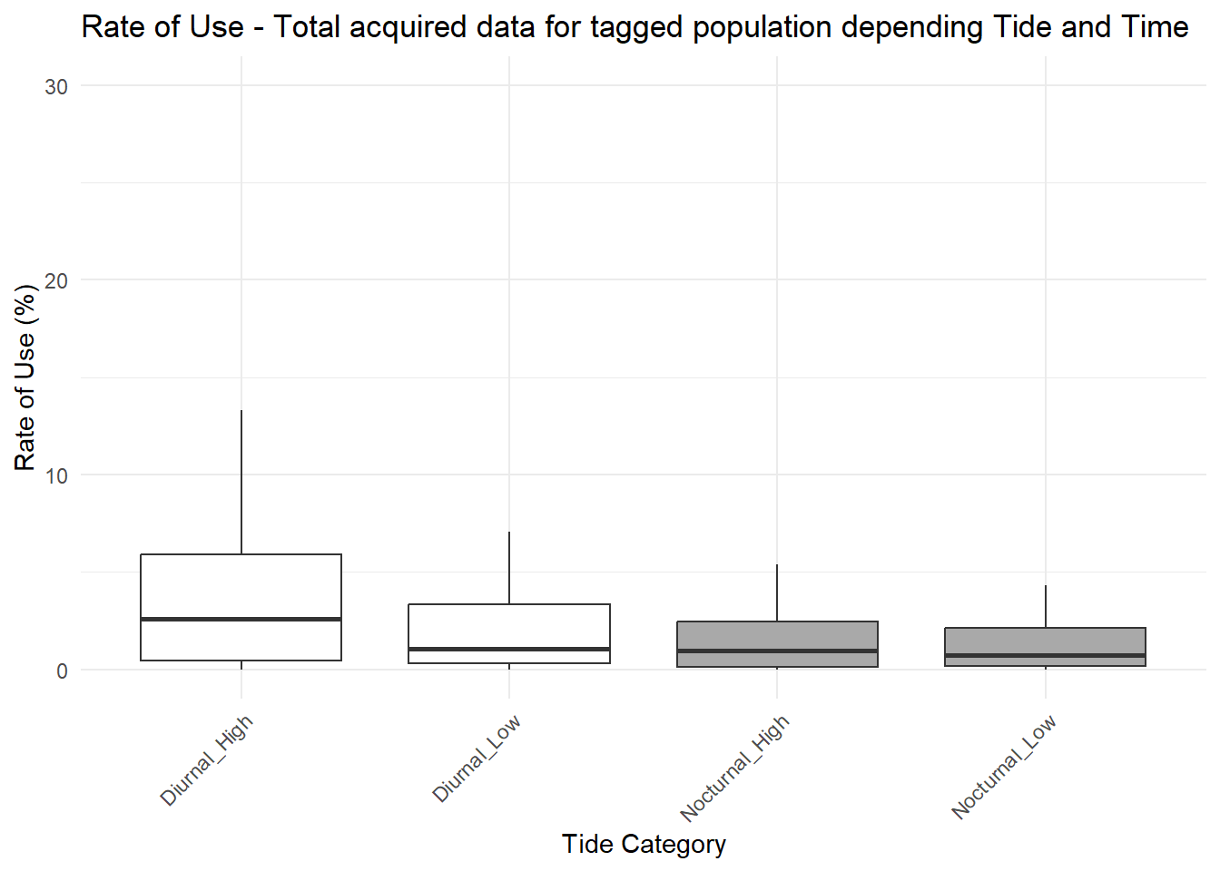
Legend: Find the values of the Usage rate (or rate of use) from the whole tagged shorebirds population detected within the Motus array and for each tide category.
TOTAL DETECTED (hours) - TOTAL USED -
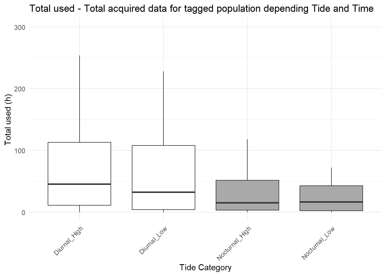
Legend: Find the total of hours (or total uses) the whole tagged shorebirds population has been recorded within the Motus array and for each tide category.
SPECIES
TOTAL SURVEY EFFORT (%) - TOTAL AVAILABLE -
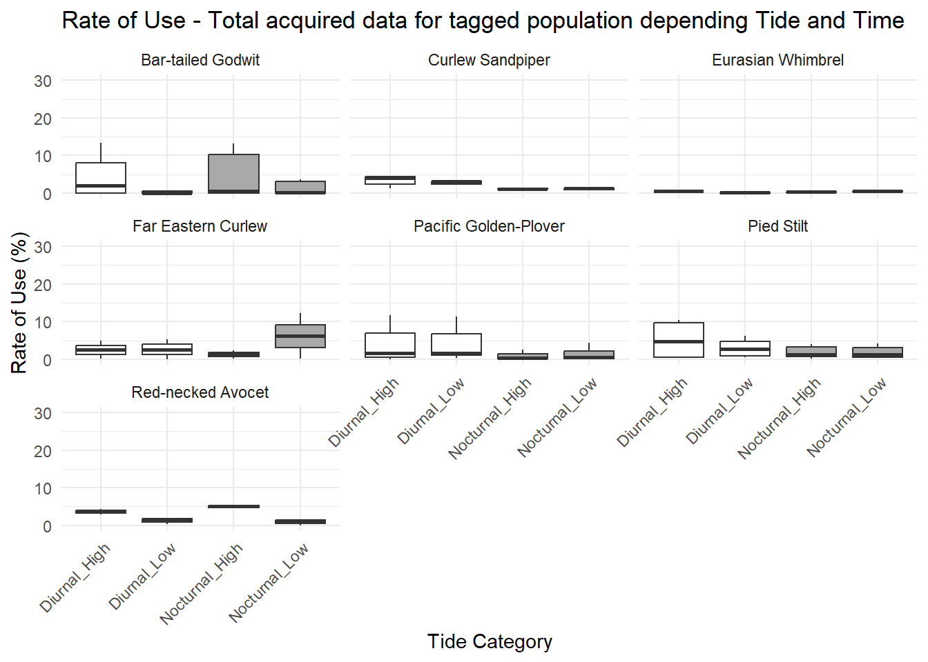
Legend: Find the values of the Usage rate (or rate of use) across each shorebirds species detected within the Motus array and for each tide category.
TOTAL DETECTED (hours) - TOTAL USED -
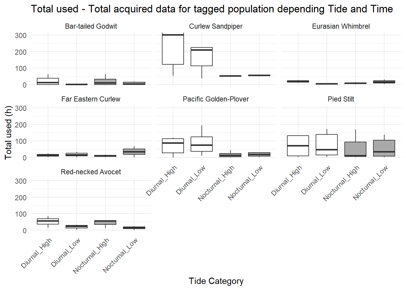
Legend: Find the total of hours (or total uses) each species has been recorded within the Motus array and for each tide category.
SITES
TOTAL DETECTED (hours) - TOTAL USED -
| Species Site Use Summary | ||||||||||
|---|---|---|---|---|---|---|---|---|---|---|
| Detected / Survey effort (Hours) per Tide Categories | ||||||||||
| N Birds | Total Hours Detected / Survey effort |
Hours per Tide Category
|
Detection per Tide Category (%)
|
|||||||
| Noct. Low | Noct. High | Diur. Low | Diur. High | Noct. Low | Noct. High | Diur. Low | Diur. High | |||
| BAR-TAILED GODWIT | ||||||||||
| Total | 10 | 508 / 72875 (0.7 %) | 69 / 18152 (0.4 %) | 198 / 18171 (1.1 %) | 22 / 18252 (0.1 %) | 219 / 18300 (1.2 %) | 13.6 | 39 | 4.3 | 43.1 |
| Curlew Point | 6 | 316 / 14445 (2.2 %) | 35 / 3525 (1 %) | 52 / 3409 (1.5 %) | 22 / 3684 (0.6 %) | 207 / 3827 (5.4 %) | 11.1 | 16.5 | 7 | 65.5 |
| Fullerton Entrance | 9 | 6 / 22641 (0 %) | 2 / 5723 (0 %) | 1 / 5819 (0 %) | < 1 / 5589 (0 %) | 3 / 5510 (0.1 %) | 33.3 | 16.7 | 0 | 50 |
| Milhams Pond | 2 | 0 / 22943 (0 %) | < 1 / 5801 (0 %) | < 1 / 5899 (0 %) | < 1 / 5658 (0 %) | < 1 / 5585 (0 %) | NaN | NaN | NaN | NaN |
| Tomago | 5 | 186 / 12846 (1.4 %) | 32 / 3103 (1 %) | 145 / 3044 (4.8 %) | < 1 / 3321 (0 %) | 9 / 3378 (0.3 %) | 17.2 | 78 | 0 | 4.8 |
| CURLEW SANDPIPER | ||||||||||
| Total | 5 | 2429 / 63678 (3.8 %) | 255 / 14154 (1.8 %) | 215 / 12306 (1.7 %) | 815 / 17550 (4.6 %) | 1144 / 19668 (5.8 %) | 10.5 | 8.9 | 33.6 | 47.1 |
| Curlew Point | 5 | 2402 / 10613 (22.6 %) | 240 / 2359 (10.2 %) | 208 / 2051 (10.1 %) | 814 / 2925 (27.8 %) | 1140 / 3278 (34.8 %) | 10 | 8.7 | 33.9 | 47.5 |
| Fullerton Entrance | 5 | 4 / 10613 (0 %) | 4 / 2359 (0.2 %) | < 1 / 2051 (0 %) | < 1 / 2925 (0 %) | < 1 / 3278 (0 %) | 100 | 0 | 0 | 0 |
| Milhams Pond | 3 | 0 / 10613 (0 %) | < 1 / 2359 (0 %) | < 1 / 2051 (0 %) | < 1 / 2925 (0 %) | < 1 / 3278 (0 %) | NaN | NaN | NaN | NaN |
| Ramsar Road | 5 | 5 / 10613 (0 %) | 3 / 2359 (0.1 %) | 2 / 2051 (0.1 %) | < 1 / 2925 (0 %) | < 1 / 3278 (0 %) | 60 | 40 | 0 | 0 |
| Swan Pond | 5 | 12 / 10613 (0.1 %) | 5 / 2359 (0.2 %) | 3 / 2051 (0.1 %) | 1 / 2925 (0 %) | 3 / 3278 (0.1 %) | 41.7 | 25 | 8.3 | 25 |
| Tomago | 5 | 6 / 10613 (0.1 %) | 3 / 2359 (0.1 %) | 2 / 2051 (0.1 %) | < 1 / 2925 (0 %) | 1 / 3278 (0 %) | 50 | 33.3 | 0 | 16.7 |
| EURASIAN WHIMBREL | ||||||||||
| Total | 2 | 96 / 7710 (1.2 %) | 33 / 1779 (1.9 %) | 16 / 1428 (1.1 %) | 9 / 2052 (0.4 %) | 38 / 2451 (1.6 %) | 34.4 | 16.7 | 9.4 | 39.6 |
| Curlew Point | 2 | 65 / 2570 (2.5 %) | 32 / 593 (5.4 %) | 15 / 476 (3.2 %) | 7 / 684 (1 %) | 11 / 817 (1.3 %) | 49.2 | 23.1 | 10.8 | 16.9 |
| Fullerton Entrance | 2 | 29 / 2570 (1.1 %) | < 1 / 593 (0 %) | < 1 / 476 (0 %) | 2 / 684 (0.3 %) | 27 / 817 (3.3 %) | 0 | 0 | 6.9 | 93.1 |
| Tomago | 1 | 2 / 2570 (0.1 %) | 1 / 593 (0.2 %) | 1 / 476 (0.2 %) | < 1 / 684 (0 %) | < 1 / 817 (0 %) | 50 | 50 | 0 | 0 |
| FAR EASTERN CURLEW | ||||||||||
| Total | 2 | 144 / 2439 (5.9 %) | 69 / 552 (12.5 %) | 17 / 646 (2.6 %) | 33 / 666 (5 %) | 25 / 575 (4.3 %) | 47.9 | 11.8 | 22.9 | 17.4 |
| Curlew Point | 1 | 1 / 313 (0.3 %) | < 1 / 68 (0 %) | < 1 / 74 (0 %) | < 1 / 88 (0 %) | 1 / 83 (1.2 %) | 0 | 0 | 0 | 100 |
| Fullerton Entrance | 2 | 0 / 859 (0 %) | < 1 / 196 (0 %) | < 1 / 236 (0 %) | < 1 / 234 (0 %) | < 1 / 193 (0 %) | NaN | NaN | NaN | NaN |
| Milhams Pond | 1 | 141 / 954 (14.8 %) | 68 / 220 (30.9 %) | 16 / 262 (6.1 %) | 33 / 256 (12.9 %) | 24 / 216 (11.1 %) | 48.2 | 11.3 | 23.4 | 17 |
| Tomago | 1 | 2 / 313 (0.6 %) | 1 / 68 (1.5 %) | 1 / 74 (1.4 %) | < 1 / 88 (0 %) | < 1 / 83 (0 %) | 50 | 50 | 0 | 0 |
| MASKED LAPWING | ||||||||||
| Total | 1 | 0 / 721 (0 %) | < 1 / 168 (0 %) | < 1 / 133 (0 %) | < 1 / 192 (0 %) | < 1 / 228 (0 %) | NaN | NaN | NaN | NaN |
| Curlew Point | 1 | 0 / 721 (0 %) | < 1 / 168 (0 %) | < 1 / 133 (0 %) | < 1 / 192 (0 %) | < 1 / 228 (0 %) | NaN | NaN | NaN | NaN |
| PACIFIC GOLDEN-PLOVER | ||||||||||
| Total | 14 | 4819 / 150283 (3.2 %) | 633 / 33472 (1.9 %) | 498 / 32839 (1.5 %) | 1797 / 41108 (4.4 %) | 1891 / 42864 (4.4 %) | 13.1 | 10.3 | 37.3 | 39.2 |
| Curlew Point | 13 | 3094 / 19237 (16.1 %) | 342 / 4295 (8 %) | 198 / 4189 (4.7 %) | 1199 / 5253 (22.8 %) | 1355 / 5500 (24.6 %) | 11.1 | 6.4 | 38.8 | 43.8 |
| Fullerton Entrance | 12 | 13 / 19237 (0.1 %) | 4 / 4295 (0.1 %) | 4 / 4189 (0.1 %) | 3 / 5253 (0.1 %) | 2 / 5500 (0 %) | 30.8 | 30.8 | 23.1 | 15.4 |
| Hexham Swamp | 11 | 330 / 19237 (1.7 %) | 19 / 4295 (0.4 %) | 36 / 4189 (0.9 %) | 149 / 5253 (2.8 %) | 126 / 5500 (2.3 %) | 5.8 | 10.9 | 45.2 | 38.2 |
| Milhams Pond | 8 | 1346 / 19237 (7 %) | 255 / 4295 (5.9 %) | 248 / 4189 (5.9 %) | 439 / 5253 (8.4 %) | 404 / 5500 (7.3 %) | 18.9 | 18.4 | 32.6 | 30 |
| Ramsar Road | 10 | 29 / 19237 (0.2 %) | 12 / 4295 (0.3 %) | 7 / 4189 (0.2 %) | 7 / 5253 (0.1 %) | 3 / 5500 (0.1 %) | 41.4 | 24.1 | 24.1 | 10.3 |
| Swan Pond | 12 | 4 / 19237 (0 %) | < 1 / 4295 (0 %) | 3 / 4189 (0.1 %) | < 1 / 5253 (0 %) | 1 / 5500 (0 %) | 0 | 75 | 0 | 25 |
| Tomago | 1 | 0 / 19237 (0 %) | < 1 / 4295 (0 %) | < 1 / 4189 (0 %) | < 1 / 5253 (0 %) | < 1 / 5500 (0 %) | NaN | NaN | NaN | NaN |
| Windeyers | 7 | 3 / 15624 (0 %) | 1 / 3407 (0 %) | 2 / 3516 (0.1 %) | < 1 / 4337 (0 %) | < 1 / 4364 (0 %) | 33.3 | 66.7 | 0 | 0 |
| PIED STILT | ||||||||||
| Total | 6 | 1746 / 114107 (1.5 %) | 333 / 29164 (1.1 %) | 314 / 28625 (1.1 %) | 441 / 27789 (1.6 %) | 658 / 28529 (2.3 %) | 19.1 | 18 | 25.3 | 37.7 |
| Curlew Point | 4 | 58 / 15271 (0.4 %) | 5 / 3792 (0.1 %) | 3 / 3561 (0.1 %) | 2 / 3823 (0.1 %) | 48 / 4095 (1.2 %) | 8.6 | 5.2 | 3.4 | 82.8 |
| Fullerton Entrance | 5 | 1031 / 24611 (4.2 %) | 187 / 6320 (3 %) | 137 / 6241 (2.2 %) | 250 / 5968 (4.2 %) | 457 / 6082 (7.5 %) | 18.1 | 13.3 | 24.2 | 44.3 |
| Milhams Pond | 1 | 20 / 24801 (0.1 %) | < 1 / 6368 (0 %) | 1 / 6293 (0 %) | 12 / 6012 (0.2 %) | 7 / 6128 (0.1 %) | 0 | 5 | 60 | 35 |
| Ramsar Road | 2 | 566 / 24525 (2.3 %) | 130 / 6300 (2.1 %) | 159 / 6211 (2.6 %) | 154 / 5942 (2.6 %) | 123 / 6072 (2 %) | 23 | 28.1 | 27.2 | 21.7 |
| Swan Pond | 2 | 71 / 24899 (0.3 %) | 11 / 6384 (0.2 %) | 14 / 6319 (0.2 %) | 23 / 6044 (0.4 %) | 23 / 6152 (0.4 %) | 15.5 | 19.7 | 32.4 | 32.4 |
| RED-NECKED AVOCET | ||||||||||
| Total | 3 | 378 / 8946 (4.2 %) | 39 / 2058 (1.9 %) | 128 / 1668 (7.7 %) | 57 / 2388 (2.4 %) | 154 / 2832 (5.4 %) | 10.3 | 33.9 | 15.1 | 40.7 |
| Curlew Point | 3 | 46 / 1491 (3.1 %) | 1 / 343 (0.3 %) | 2 / 278 (0.7 %) | 2 / 398 (0.5 %) | 41 / 472 (8.7 %) | 2.2 | 4.3 | 4.3 | 89.1 |
| Fullerton Entrance | 3 | 244 / 1491 (16.4 %) | 19 / 343 (5.5 %) | 67 / 278 (24.1 %) | 55 / 398 (13.8 %) | 103 / 472 (21.8 %) | 7.8 | 27.5 | 22.5 | 42.2 |
| Hexham Swamp | 2 | 0 / 1491 (0 %) | < 1 / 343 (0 %) | < 1 / 278 (0 %) | < 1 / 398 (0 %) | < 1 / 472 (0 %) | NaN | NaN | NaN | NaN |
| Milhams Pond | 2 | 0 / 1491 (0 %) | < 1 / 343 (0 %) | < 1 / 278 (0 %) | < 1 / 398 (0 %) | < 1 / 472 (0 %) | NaN | NaN | NaN | NaN |
| Swan Pond | 2 | 1 / 1491 (0.1 %) | 1 / 343 (0.3 %) | < 1 / 278 (0 %) | < 1 / 398 (0 %) | < 1 / 472 (0 %) | 100 | 0 | 0 | 0 |
| Tomago | 3 | 87 / 1491 (5.8 %) | 18 / 343 (5.2 %) | 59 / 278 (21.2 %) | < 1 / 398 (0 %) | 10 / 472 (2.1 %) | 20.7 | 67.8 | 0 | 11.5 |
Legend: Summary for each species and per Motus station of the number of hours a species has been detected and the number of hours the station has been listening while the species had at least one individual with an activated tag on (survey effort). NA are when the group holds individuals that are detected less than one hour total.
The only remaining limitation is the high number of hours sharing the same date and time across several Motus stations, for the survey effort. Which is not realistic since the birds can be at only one place at once.