Estuary usage - days

Published

2026-03-06

Birds remain within the same estuaries. Migratory ones during all summer and residents all year around. That’s a statement at species group level. But do the individuals remain within the same estuary or do they fly from one to another?

To address this question we’ll quantify how many days a bird has been detected at least once on at least one Motus station in one estuary, and we’ll put this number of days against the total number of day that same bird was detectable. The result will be expressed in percentage.

Variables

Load your data in your R environment - see Load & Format > Reproducibility

library(dplyr)
library(here) 
library(ggplot2)
library(lubridate)
library(tidyr)

Let’s count days and detecting stations for each bird.

# Get deployment duration for each tags (in days)
tag_dep_duration <- data_all %>%
  group_by(Band.ID) %>%
  summarise(start_date = min(DateAUS.Trap),
            end_date = max(dateAus),
            period_tag_dep_d = 1 + time_length(interval(start = start_date, end = end_date), unit = "day"), # +1 to include the trapping day
            .groups = "drop") %>%
  select(Band.ID, period_tag_dep_d)

# Get number days each tag has been detected at least once in any station
tag_dep_nb_d <- data_all %>%
  mutate(dateAus = as.Date(dateAus)) %>%
  group_by(Band.ID) %>%
  summarise(days_detect = n_distinct(dateAus), .groups = "drop")

# Get number of days one tag has been recorded in >1 station (for each tags)
multiple_site_detect <- data_all %>%
  group_by(Band.ID, dateAus) %>%
  # Counts per day the number of station one tag has been recorded
  summarise(distinct_sites = n_distinct(recvDeployName),
            .groups = "drop_last") %>%
  # Tells if one day one tag has been recorded several sites
  mutate(multiple_detect = distinct_sites > 1) %>%
  group_by(Band.ID) %>%
  summarise(multiple_site_detect = sum(multiple_detect),
            .groups = "drop")

We generate tag_dep_duration that counts the total of days period_tag_dep_d each bird Band.ID had a tag on and activated. We make tag_dep_nb_d that quantifies the number of days days_detect each bird have been detected at least once in the Motus array.

So, we can then compare the first value with the second, and obtain our metric of interest in percentage.

Additionally, we quantified in multiple_site_detect the number of days each bird has been detected in multiple stations.

Results

INDIVIDUALS

# Get number of day each tag has been recorded /species and /station
tag_detection_indiv <- data_all %>%
  group_by(Band.ID, recvDeployName, speciesEN) %>%
  # to count sp*ID per recv
  reframe(days_recorded = n_distinct(dateAus)) %>%
  # flip table to get one column per station
  pivot_wider(names_from = recvDeployName, 
              values_from = days_recorded,
              values_fill = 0) %>% # = 0 if NA
  left_join(multiple_site_detect, by = "Band.ID") %>%
  left_join(tag_dep_nb_d, by = "Band.ID") %>%
  left_join(tag_dep_duration, by = "Band.ID") %>%
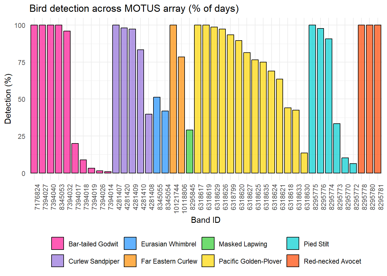
  mutate(perc = round((days_detect / period_tag_dep_d) * 100, 1)) # nb of day one tag is recorded once / nb of day the tag is deployed

The above table presents daily detection for each bird and for each Motus station in the local array:

multiple_site_detect: number of days a bird has been detected in more than one station
days_detect: number of days a bird has been detected in at least one station
period_tag_dep_d: total of days a bird was detectable with a tag on and activated
perc: (days_detect / period_tag_dep_d) x 100

Visualise below for each birds the number of days the individual has been detected at least once and in at least one Motus station in the array, against the total of days the bird had a tag on and activated (results in %).

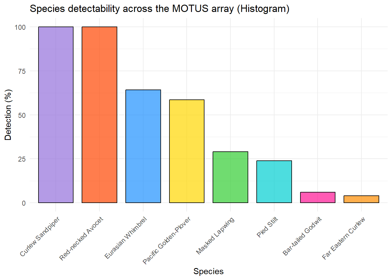
SPECIES

Below are the same results as above, but for each species. So the data has been grouped by species.

speciesEN	Curlew Point	Fullerton Entrance	Hexham Swamp	Milhams Pond	Ramsar Road	Swan Pond	Tomago	Windeyers	multiple_site_detect	days_detect	period_tag_dep_d	perc
Bar-tailed Godwit	48	50	0	5	0	0	22	0	43	64	1064	6.0
Curlew Sandpiper	106	52	0	7	62	107	65	0	107	111	111	100.0
Eurasian Whimbrel	36	22	0	0	0	0	9	0	16	50	78	64.1
Far Eastern Curlew	1	25	0	22	0	0	12	0	17	43	1078	4.0
Masked Lapwing	9	0	0	0	0	0	0	0	0	9	31	29.0
Pacific Golden-Plover	219	77	51	77	76	96	1	17	158	280	478	58.6
Pied Stilt	18	105	0	2	69	61	0	0	68	159	664	23.9
Red-necked Avocet	24	29	3	4	0	5	21	0	29	29	29	100.0

ggplot(tag_detection_indiv %>%
         add_count(speciesEN) %>%
         mutate(species_label = paste0(speciesEN, " (n = ", n, ")")),
       aes(x = reorder(species_label, -perc, FUN = median),
           y = perc, fill = speciesEN)) +   
  geom_boxplot(width = 0.8, alpha = 0.7, color = "black") +
  scale_fill_manual(values = species_colors) +
  theme_minimal() +
  theme(axis.text.x = element_text(angle = 45, hjust = 1),
        legend.position = "none") +
  labs(x = "Species (n = number of individuals)",
       y = "Detection (%)",
       title = "Species detectability across the MOTUS array (Boxplot)")

detection_table <- tag_detection_indiv %>%
  add_count(speciesEN) %>%
  mutate(Species = speciesEN) %>%
  group_by(Species, speciesEN) %>%
  summarise(
    n_individuals = n(),
    min = round(min(perc, na.rm = TRUE), 1),
    q1 = round(quantile(perc, 0.25, na.rm = TRUE),1),
    median = round(median(perc, na.rm = TRUE),1),
    q3 = round(quantile(perc, 0.75, na.rm = TRUE),1),
    max = round(max(perc, na.rm = TRUE),1),
    mean = round(mean(perc, na.rm = TRUE),1),
    sd = round(sd(perc, na.rm = TRUE),1),
    .groups = 'drop'
  ) %>%
  arrange(desc(median)) %>%
  select(-speciesEN)

library(gt)
detection_table  %>%
  gt() %>%
  opt_align_table_header(align = "left")  %>%
  tab_style(
    style = cell_text(weight = "bold"),
    locations = cells_column_labels() ) %>%
  tab_style(
    style = cell_text(style = "italic"),
    locations = cells_body(columns = c(Species)))

Species	n_individuals	min	q1	median	q3	max	mean	sd
Red-necked Avocet	3	100.0	100.0	100.0	100.0	100.0	100.0	0.0
Curlew Sandpiper	5	39.7	83.3	97.3	98.2	100.0	83.7	25.5
Far Eastern Curlew	2	78.4	83.8	89.2	94.6	100.0	89.2	15.3
Pacific Golden-Plover	14	13.6	65.0	79.0	96.4	100.0	74.7	26.1
Pied Stilt	6	6.3	16.0	62.0	96.0	100.0	56.4	44.7
Bar-tailed Godwit	10	0.8	4.7	58.0	100.0	100.0	53.0	49.0
Eurasian Whimbrel	2	41.9	44.2	46.6	48.9	51.3	46.6	6.6
Masked Lapwing	1	29.0	29.0	29.0	29.0	29.0	29.0	NA