Survey effort

One key element we must address in our study is to define when and for how long each Motus station in our array was operational and thus able to detect VHF-tagged birds?

Stations may have operated for varying duration or during different time periods, making raw detection counts inherently biased and non-comparable. By quantifying the survey effort (total operational time) for each station, we can standardise the results across stations and allow statistically valid comparisons, ensuring that observed differences reflect true ecological patterns rather than artifacts of unequal sampling effort.

To exactly access when a station was operational and when it was not, we used the activity table coming from each station’s receiver. This table records any VHF activity at any time.

Note: The following terms are used interchangeably: (1) receivers, SensorGnome, SG, serno, recv; (2) Raspberry Pi processor, Raspberry, deviceID.

Activity table

Load your data in your R environment - see Load & Format > Reproducibility

library(dplyr)
library(here)
library(forcats) 
library(ggplot2)
library(lubridate)
library(tidyr)
library(purrr)

Let’s call this famous activity table.

recv.act <- tbl(sql.motus, "activity")  %>% 
  collect() %>% 
  as.data.frame() %>%
  rename(deviceID = "motusDeviceID") %>%
  # keep our deployed antennas only
  filter(deviceID %in% unique(recv$deviceID)) %>% 
  # Set the time properly - IMPORTANT
  mutate(date = as_datetime(as.POSIXct(hourBin* 3600,
                                       origin = "1970-01-06", 
                                       tz = "UTC")),
         dateAus = as_datetime(as.POSIXct(hourBin* 3600, 
                                          origin = "1970-01-06", 
                                          tz = "UTC"), 
                               tz = "Australia/Sydney"))   

head(recv.act)

   batchID deviceID ant hourBin numTags pulseCount numRuns numHits run2 run3
1 21275568     3596   1  471533       1         20       1       9    0    0
2 21275568     3596   1  471534       0         46       0      NA    0    0
3 21275568     3596   1  471535       0         79       0      NA    0    0
4 21275568     3596   1  471536       0          8       0      NA    0    0
5 21275568     3596   1  471537       0         23       0      NA    0    0
6 21275568     3596   1  471538       0          6       0      NA    0    0
  run4 run5 run6 run7plus numGPSfix                date             dateAus
1    0    0    0        1        NA 2023-10-22 05:00:00 2023-10-22 16:00:00
2    0    0    0        0        NA 2023-10-22 06:00:00 2023-10-22 17:00:00
3    0    0    0        0        NA 2023-10-22 07:00:00 2023-10-22 18:00:00
4    0    0    0        0        NA 2023-10-22 08:00:00 2023-10-22 19:00:00
5    0    0    0        0        NA 2023-10-22 09:00:00 2023-10-22 20:00:00
6    0    0    0        0        NA 2023-10-22 10:00:00 2023-10-22 21:00:00

Here above is displayed an overview of the activity table. This object is composed of multiple elements but four are keys:

• pulseCount: Quantifies the number of radio pulses measured on each antenna over each hour period hourBin but does not necessary correspond to a known VHF tag detection. It can be any other VHF signal, even simple noise - documentation
• numTags: Represents the total number of unique tags detected. This, given a context, as typically a specific site, or within a batch, or for a set of detections.
• deviceID: Raspberry Pi processor ID. A small electronic part of the receiver that plays the role of an embarked computer.
• ant: Port of antenna the activity has been recorded.

How the data are recorded in this table?

Two cases may occur:

• When a station is listening, the table has either values or NA for pulseCount or/and for numTags variables. For example:

  • No noise has been recorded but one or several tags have been recorded: pulseCount = 0 or is NA and numTags > 1

  • No tag has been recorded but noise happened: pulseCount > 0 and numTags = 0 or is NA

• When a station is not listening, there is no row at all in the table (no data recorded).

Keep in mind we can miss the hours where no tag or noise are happening within the environment BUT the antenna is still operational and being “listening”. In such a case, let’s further assume than the antenna is not working or listening. Indeed, an environment with “no noise” condition during more than an hour may be extremely rare and very unlikely.

table(is.na(recv.act$pulseCount), recv.act$numTags) 

       
             0      1      2      3      4      5      6      7     13     14
  FALSE 126304   5823   1329    661    289    125     40     17      1      1
  TRUE   13191    138     32      7      2      2      0      0      0      0
       
            16
  FALSE      2
  TRUE       0

Receiver ID

One issue with Motus data is the number of variables related to IDs (receivers, Raspberry Pi, sites, etc.) and the inconsistent use of names for the same variable across the different tables (i.e. recv$serno = data_all$recv).

Plus, some of our SensorGnome serno and/or Raspberry Pi processor deviceID have been swapped around stations to optimise the VHF survey.

For example, when two stations need receiver repairs, we fix the easiest one first and prioritise reinstalling it at the most important station regardless the receiver or Raspberry origin. This sometimes means taking a receiver or Raspberry from one station and moving it to another one, but because Motus attaches this Raspberry ID deviceID to a Motus station name recvDeployName, messy error may happen.

We must re-associate each deviceID with their corresponding recvDeployName and at the correct hourBin. We first create a unique ID that matches station’s name with Raspberry pi that we called SernoStation.

# Sort the terminated serno (if terminated, ie. one box has been removed from one antenna site, and a date comes along recv$timeEndAus variable)
recv.act.term <- recv.act %>%
  left_join(recv %>% 
              filter(!is.na(timeEndAus)) %>%
              select(deviceID, serno, recvDeployName),
            "deviceID") %>%
  filter(!is.na(recvDeployName)) %>%
  mutate(SernoStation = paste0(recvDeployName, "_", serno))

# Sort the still currently running serno
recv.act.runn <- recv.act %>%
  left_join(recv %>% 
              filter(is.na(timeEndAus)) %>%
              select(deviceID, serno, recvDeployName),
            "deviceID") %>%
  filter(!is.na(recvDeployName)) %>%
  mutate(SernoStation = paste0(recvDeployName, "_", serno))

# Merging in one data-set to use Station's name further + pick-up the rounded hours
recv.act <- bind_rows(recv.act.runn, recv.act.term) %>%
  mutate(hour_dt = floor_date(dateAus, "hour"))

# Providing helpful variables
recv <- recv %>%
  mutate(SernoStation = paste0(recvDeployName, "_", serno),
         lisStart = timeStartAus,
         lisEnd = if_else(
           is.na(timeEndAus), # means the station is still running since the last data downloading
           with_tz(Sys.time(), "Australia/Sydney"),
           with_tz(as_datetime(timeEndAus, tz = "UTC"), "Australia/Sydney")) )

We get recv.act table with every rows of activity the variables lisStart and lisEnd that specifies the complete period of time the station recvDeployName has been deployed with what deviceID.

When a station is still deployed, lisEnd = NA.

Operational periods

# Generating hourly sequences per SernoStation from start to end dates of the deviceID at particular sites
recv_hours <- recv %>%
  select(recvDeployName, deviceID, SernoStation, lisStart, lisEnd) %>%
  rowwise() %>%
  mutate(hour_dt = list(seq(from = floor_date(lisStart, unit = "hour"),
                            to = floor_date(lisEnd, unit = "hour"),
                            by = "hour")) ) %>%
  unnest(cols = c(hour_dt)) %>%
  ungroup()

# Giving operational and not-operational hours by joining same sequences from recv.act tbl and adding operational = TRUE when existing values
recv_hours <- recv_hours %>%
  left_join(recv.act %>%
              distinct(SernoStation, hour_dt) %>%
              mutate(operational = TRUE),
            by = c("SernoStation", "hour_dt")) %>%
  mutate(operational = if_else(is.na(operational), FALSE, TRUE))

# Relaying on the Station name on its own only (consistent values through SernoStation var)
recv.act$Station <- sub("_SG-.*", "", recv.act$SernoStation)
recv$Station <- sub("_SG-.*", "", recv$SernoStation)
recv_hours$Station <- sub("_SG-.*", "", recv_hours$SernoStation)

This step runs for each row of each recv and creates one list composed of as many rows of as many hours it is contained within the period [lisStart - lisEnd].

If lisEnd is NA because the station is still running, the date of today is taken.

This prepares the recv_hours table where each row is one hour when one station SernoStation is potentially operational and listening.

Operational hours: To get the operational hours for each stations, meaning “when a station is actually listening”, we first gave an extra variable to the recv.act table when operational is always TRUE to records only the hours when the station is listening. These rows are the hours where one site is deployed and operational.

Non-operational hours: And we join this to the recv table by the shared variable hour_dt, which then will generate NA for the cases recv_hours$hour_dt has no matching values with recv.act$hour_dt. These NA are the hours where one site is deployed, but not operational.

Finally, for consistency, we make sure that we are using station’s name (Station) regardless the deviceID since this one might have been swapped around (see Receiver ID).

Survey effort

STATISTICS

uptime_summary <- recv_hours %>%
  group_by(Station) %>%
  summarise(
    total_hours = n(),
    operational_hours = sum(operational), 
    downtime_hours = total_hours - operational_hours, 
    uptime_pct = round(100 * operational_hours / total_hours), 2)  %>% 
  mutate(cont_listening_eff = round(100 * operational_hours / sum(operational_hours), 1), 
         surv_time_cover = round(100 * operational_hours / total_hours, 1)) %>%
  arrange(desc(uptime_pct)) %>%
  select(-c("2"))

Station	total_hours	operational_hours	downtime_hours	uptime_pct	cont_listening_eff	surv_time_cover
Swan Pond	25982	24248	1734	93	19.6	93.3
Hexham Swamp	21772	17058	4714	78	13.8	78.3
Corrie Island	20922	15218	5704	73	12.3	72.7
Ramsar Road	25815	18216	7599	71	14.8	70.6
Fullerton Entrance	25743	17221	8522	67	13.9	66.9
Milhams Pond	25934	13144	12790	51	10.6	50.7
Curlew Point	21772	10813	10959	50	8.8	49.7
Tomago	20870	6673	14197	32	5.4	32.0
Windeyers	10743	441	10302	4	0.4	4.1
Davies Point	20892	441	20451	2	0.4	2.1
Dudley Test Site	4142	0	4142	0	0.0	0.0

• total_hours: total of hours for the station being deployed into the field, regardless whether it is working/listening
• operational_hours: total of hours for the station being listening, regardless the deviceID
• downtime_hours: total of hours for the station being NOT listening, regardless the deviceID
• uptime_pct: per station, percentage of being listening over its total_hours
• cont_listening_eff: per station, contribution (%) of hours being listening (operational_hour) over the total (sum) of listening period across all the stations
• surv_time_cover: per station, temporal coverage (%) of hours being listening (operational_hour) over the period of time the array has been deployed (i.e. from the first day the first deployed station has been listening to the last day the last deployed station has been listening)

THE ARRAY

Warning: Removed 15 rows containing missing values or values outside the scale range
(`geom_segment()`).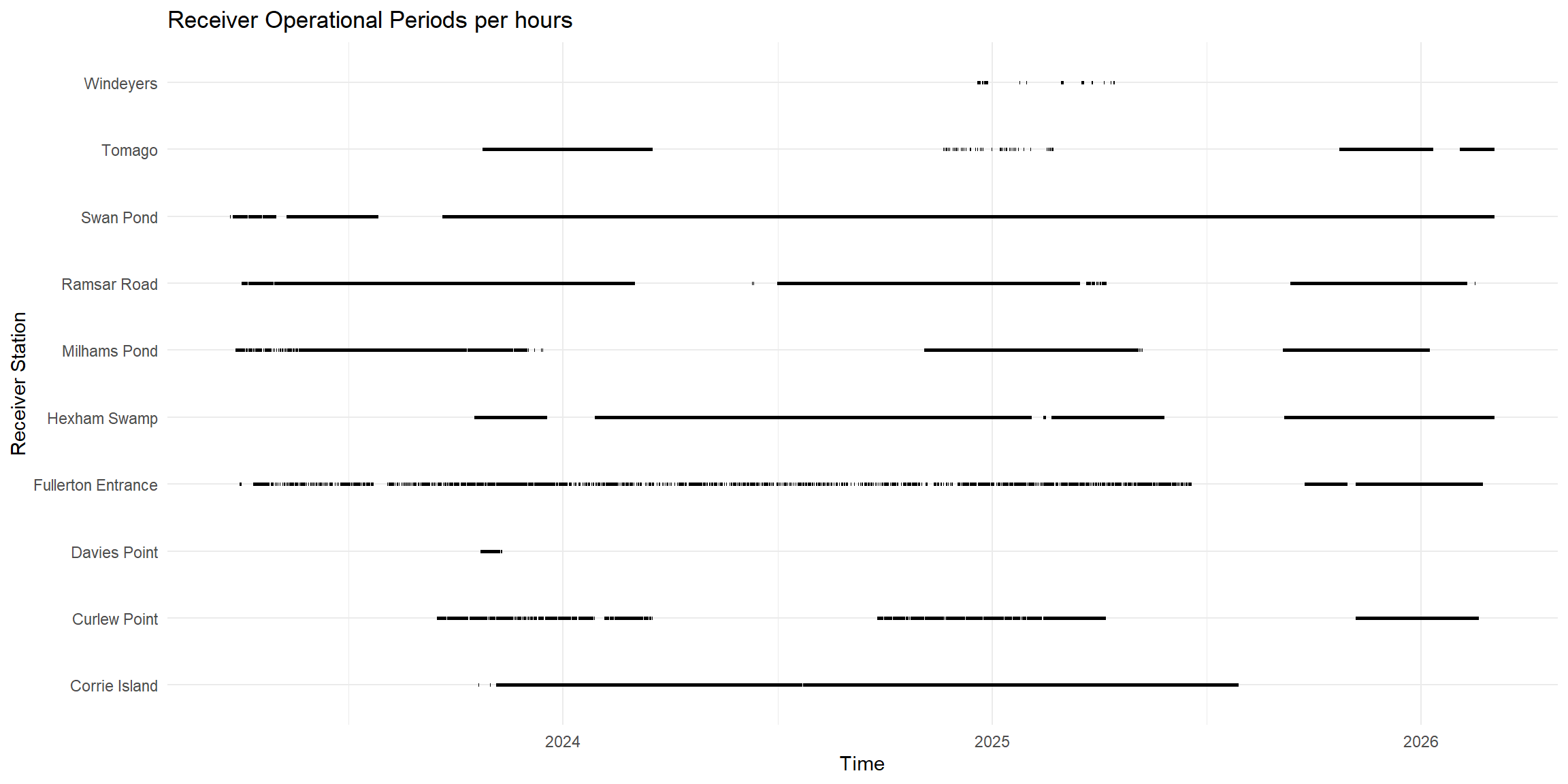

Every black dot represent an hour where the station has activity recorded meaning the station is operational, meaning recording radio noise or a specific tag.

Solid black lines are when a MOTUS station is operational. To simplify, when a station is not operational less than 24 hours, this period is considered as a operational period. Every dot represent at least one detection of one bird within an hour of the operational period. Every MOTUS station has a contribution value at the survey effort (%), i.e: Curlew Point station contributed 8.8 % to the total operational period for every stations within our local MOTUS array.

STATIONS

Curlew Point (8.8%)

Fullerton Entrance (13.9%)

Hexham Swamp (13.8%)

Milhams Pond (10.6%)

Ramsar Road (14.8%)

Swan Pond (19.6%)

Tomago (5.4%)

Windeyers (0.4%)

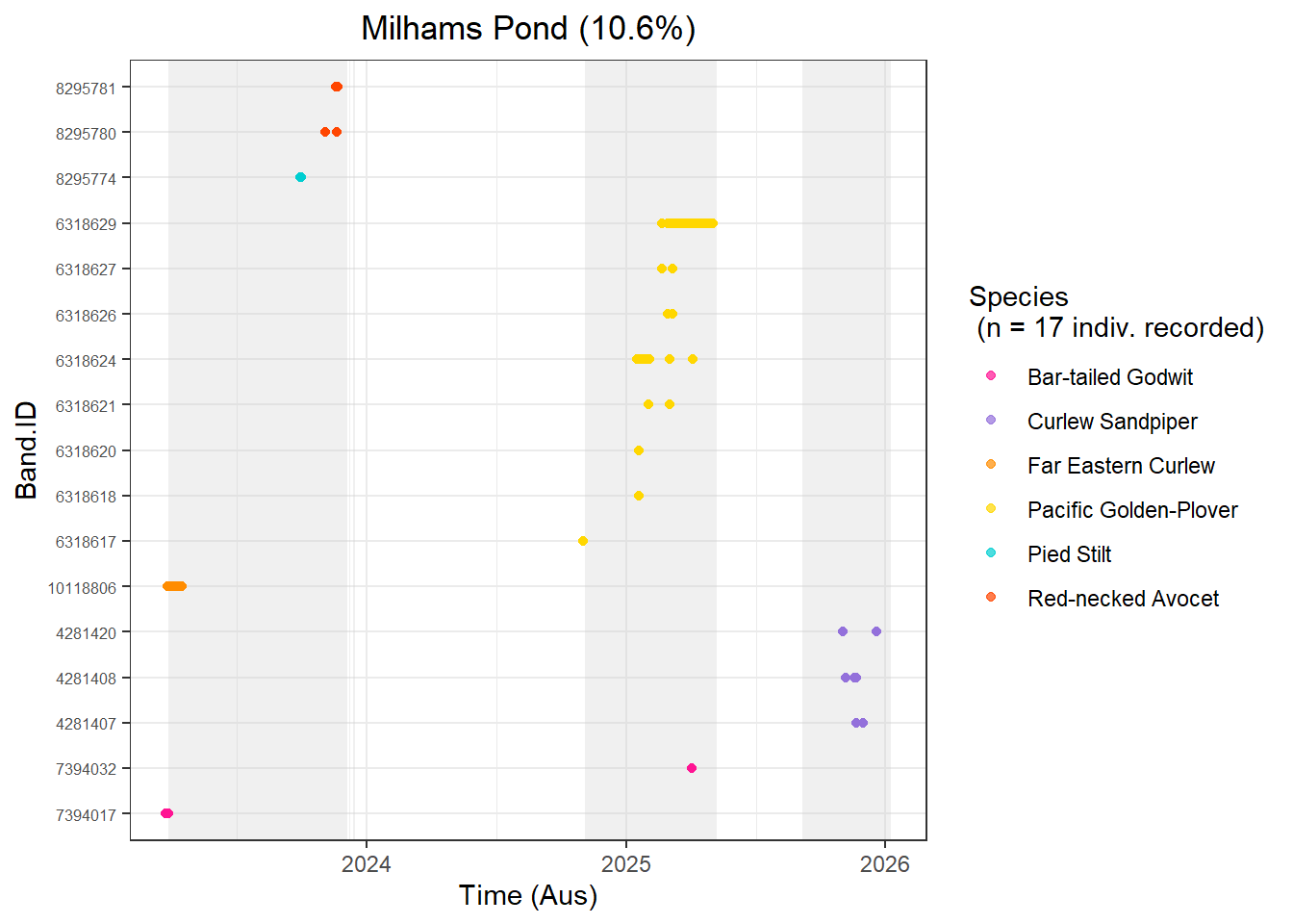
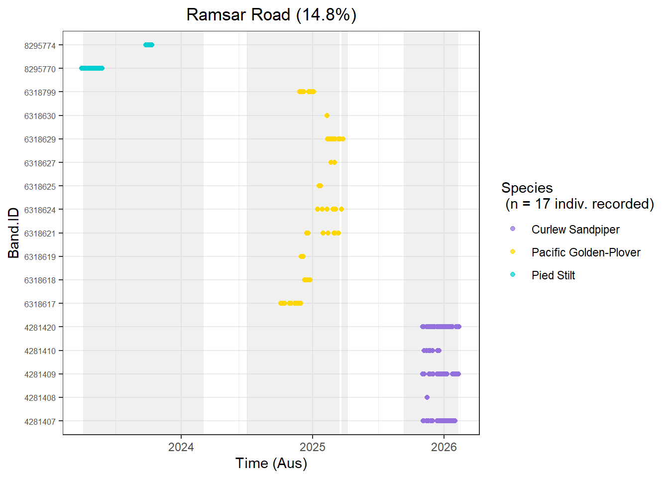
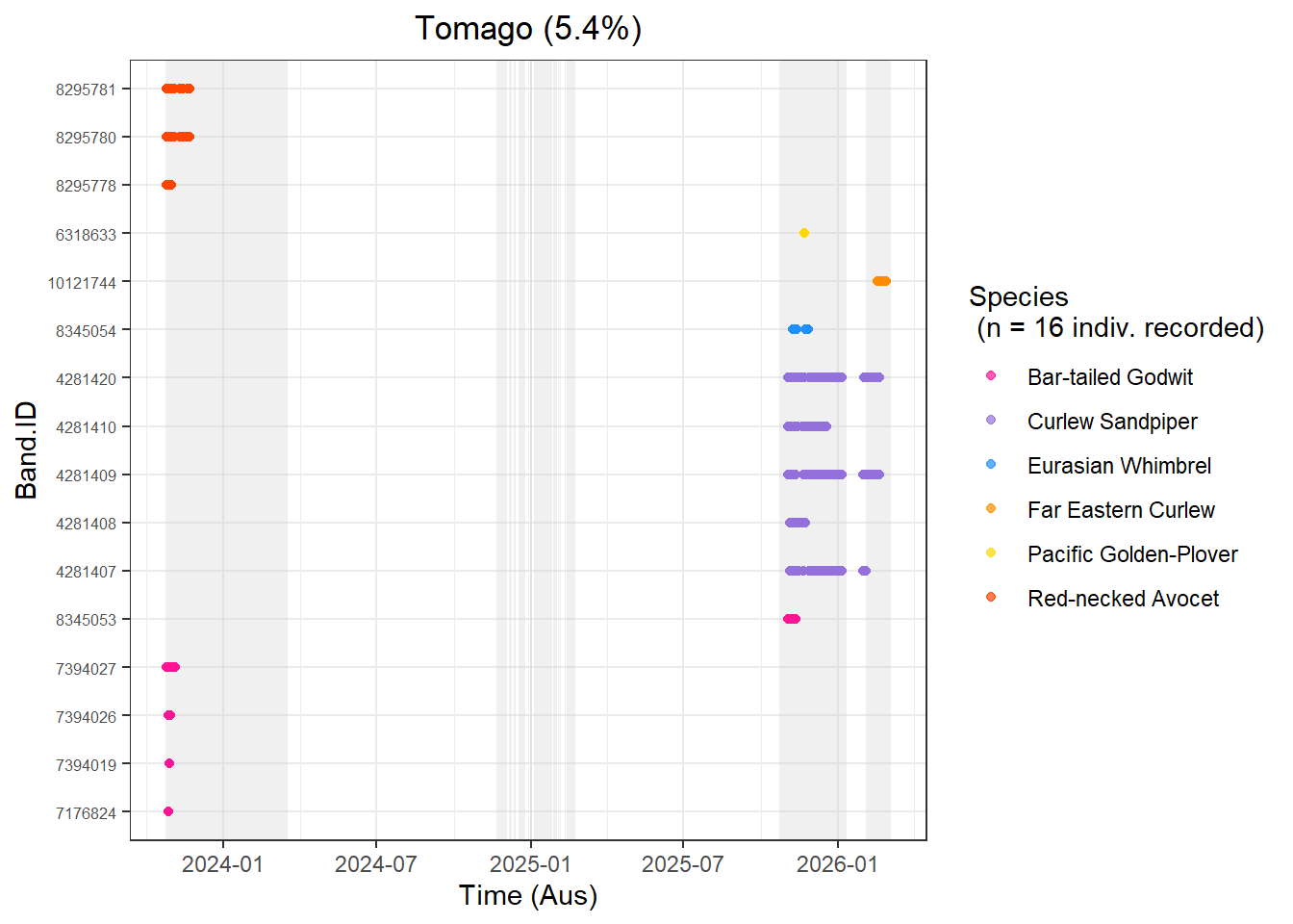
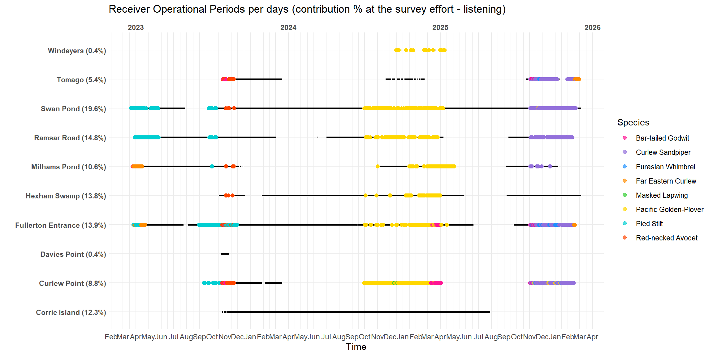
Legend: The band in grey represents the operational period for each MOTUS station, when the antenna is actually listening. When no grey, the station is “OFF” and not operational. Every dot is at least one detection for one tag. Every MOTUS station has a contribution value at the survey effort (%), i.e: Curlew Point station contributed 8.8 % at the total operational period for every stations within our local MOTUS array (operational survey effort).

Condition of detections

Find in Chapter 1 > Station usage - hours > Condition detections the number of hours a species have been detected and where, depending the four categories of tide (Low, High, Day, Night).